/images/avatar.png
Change Language 👉   

Farewell to the Rotating-Wave Approximation: An Exact Solution of the Quantum Rabi Model

1. Introduction

In the early days of quantum mechanics, Rabi proposed the Rabi model to treat the interaction between an electromagnetic field and an atom. Since this model quantized only the atom, rather than the electromagnetic wave, it could explain many phenomena (such as Rabi oscillations), but could not explain phenomena involving quantization of the electromagnetic field, such as spontaneous emission.

To explain spontaneous emission and other phenomena involving quantization of the electromagnetic field, Jaynes and Cummings proposed the Quantum Rabi Model (QRM) in 1962. This model also quantizes the electromagnetic field, meaning that vacuum fluctuations of the electromagnetic field cannot be neglected. Thus, spontaneous emission is simply “stimulated emission” “excited” by vacuum fluctuations of the electromagnetic field.
A Fully Quantum Theory of Lasers

Most materials introducing lasers derive them in a classical or semiclassical form. So what does a fully quantum theory of lasers look like? And what is it useful for?

This article briefly introduces the Scully-Lamb theory of lasers. It is a fully quantum theory, and since it is generally introduced only in the final chapters of quantum optics textbooks, while (semi-)classical theories work well in most cases, not many people are familiar with the Scully-Lamb theory.

The collapsed state of position measurement

Common sense tells us that an actual position measurement will not produce a delta function, as the delta function itself is pathological. So what should the collapsed state of an actual position measurement look like?


TL;DR:

Let the wave function of the system to be measured be $\varphi(x)$, then the collapsed wave function is:

$\varphi^{(q)}(x) = \mathcal{A}\psi(q-gx) \varphi(x)$

where $\psi(x)$ is the initial wave function of the instrument’s pointer. $q$ is the reading of the instrument’s pointer. $g$ is the coupling strength between the instrument and the system to be measured. $\begin{aligned} \mathcal{A} = \left[\int_\mathbb{R}\psi(q-gx) \varphi(x)\right]^{-1} \end{aligned}$ is the appropriate normalization constant.

Does the speed of quantum entanglement exceed the speed of light?

Too long; didn’t read version:

“Spooky action at a distance (superluminal)” is an outdated view. According to special relativity, there is no interaction between events at spacelike separation. The mainstream view in academia is to consider quantum states and measurement bases together as reality, known as contextuality. Nonlocality is a corollary of contextuality.


Body:

Discussing the “speed” of quantum entanglement is meaningless.

If the distance between two measurement events a and b is spacelike, then a is neither in the past nor in the future of b.

A Simple Quantum Description of Lasers

This article aims to derive, using a simple physical picture, the fact that the state output by a laser is a coherent state.

Consider the interaction between a two-level system and a single-mode optical field, with the field frequency equal to the energy-level spacing.

The two-level system initially occupies the excited state \(|e\rangle\), while the optical field is in the vacuum state \(|0\rangle\).

According to the Jaynes-Cummings model, spontaneous emission occurs even when the optical field is in the vacuum state. After a short time, the quantum state evolves from \(|e,0\rangle\) to:

Does the idler light passing through the optical fiber amplifier still entangle with the signal light?

Does the idler light passing through the optical fiber amplifier still entangle with the signal light, which is produced by SPDC?

Let’s consider two extremes:

Extreme 1: The gain of the amplifier is equal to 1, that is, there is no gain at all.

In this case, the amplifier acts as if it has done nothing and is an identity channel. So, of course, the entanglement will still be maintained. (Actually, it’s not necessarily the case. Even if the gain is zero, additional noise may be introduced, but we ignore it here for now).

Orbital Angular Momentum of Photons

Preface

A 1992 article published in PRA [1] pointed out that photons also possess orbital angular momentum (OAM). Unlike spin angular momentum (i.e., polarization, SAM, Spin Angular Momentum), which can only take \(\pm \hbar\), orbital angular momentum can take any integer multiple of \(\hbar\). Such orbital angular momentum can be carried by helically shaped wavefronts.

You may be surprised: people did not discover this until 1992? In fact, helically shaped wavefronts had already been studied before 1992; photons carrying angular momentum greater than \(\hbar\) had also long been predicted by atomic physics (except that they arise from higher-order transition processes, which do not satisfy selection rules and therefore have extremely low probabilities, making them essentially impossible to observe experimentally). It was not until 1992 that Allen et al. pointed out that beams with helically shaped wavefronts carry quantized orbital angular momentum.

How are creation and annihilation operators derived?

The motivation for defining creation and annihilation operators is simple and can be entirely derived from classical mechanics.

Think about how we solve the classical harmonic oscillator. Since position and momentum are coupled:

$\begin{cases} \frac{\mathrm{d}x}{\mathrm{d}t} = \omega p \\ \frac{\mathrm{d}p}{\mathrm{d}t} = -\omega x \end{cases}$

That is,

$\frac{\mathrm{d}}{\mathrm{d}t} \begin{bmatrix} x \\ p \end{bmatrix} = \begin{bmatrix} 0 & \omega \\ -\omega & 0 \end{bmatrix} \begin{bmatrix} x \\ p \end{bmatrix}$

So, we just need to decouple them. By diagonalizing, we obtain the eigenvectors $a^{\pm} = x \pm \mathrm{i} p$, and the derivatives of $a^{\pm}$ only depend on themselves:

The Difference Between Quantum Entanglement and Classical Correlations, and the Quantum Measurement Problem

When many physicists popularize quantum entanglement to the general public, they often give an example:

Imagine that you have two boxes, one containing a pizza and the other containing a hamburger, and you cannot know what is inside before opening them. Alice and Bob each take one box and travel to places far apart. At this point, when Alice opens her box, she can know what is in Bob’s box far away.

A Concise Introduction to Quantum Metrology

I. Introduction to Quantum Metrology

Quantum metrology is the study of using the quantum properties of quantum states for precision measurement.

The reason to study quantum metrology is that the measurement precision of any physical quantity is limited by the Heisenberg uncertainty principle in quantum mechanics; this is called the Heisenberg limit. How to approach and improve this limit is the goal of quantum metrology.

Of course, most measurements in everyday life do not need to reach the Heisenberg limit (for example, weighing oneself). However, in high-precision imaging and various high-precision scientific experiments, people have indeed long approached the Heisenberg limit.

[Quantum Optics Experiment Notes · III] Quantum State Tomography

Quantum State Tomography

Quantum state tomography is the process of inferring a quantum state from the measurement results of an ensemble of quantum states. Its formulation is very simple, as follows:

Given a set of measurement operators \(\{\Pi_1,\cdots,\Pi_n\}\) and their corresponding measurement probabilities \(p_k=\operatorname{Tr}[\rho \Pi_k]\), find the quantum state \(\rho\).

In other words, in these n equations \(p_k=\operatorname{Tr}[\rho \Pi_k]\), \(p_k\) and \(\Pi_k\) are known, and \(\rho\) is to be found.

What Is the Relationship Between Photons and Electromagnetic Field Wave Packets?

A Wave Packet Can Correspond to a Photon

Example: A photon can be in a state of coherent superposition of different frequencies: \(|\psi\rangle=\sum_{k}c_k|k\rangle,\quad \sum_k|c_k|^2=1\). In this case, the photon can manifest as a wave packet.

You can imagine an atom de-exciting and producing a photon; this photon will of course manifest as a wave packet.

Some may argue: if all nonideal factors are excluded, then the linewidth of this photon depends only on natural broadening (lifetime), and it can be regarded as having a single frequency. It therefore has poor localization and cannot be called a wave packet. This is indeed true.
However, if one considers single photons generated by pulsed pumping and parametric processes in the low-gain regime, their natural linewidth is itself very large. In this case, they are indeed in a coherent superposition of different frequencies and manifest as well-localized wave packets in the time domain.

Wave function of photons

The wave function of a photon in the spacetime representation is:

$\Psi(\mathbf{r},t)=\langle \mathbf{r},t|\psi\rangle=\langle 0 |E^{+}(\mathbf{r},t)|\psi\rangle$

Where $\begin{aligned} |\mathbf{r},t\rangle = E^{-}(\mathbf{r},t) |0\rangle = \sum_{\mathbf{k},\lambda} \sqrt{\frac{\hbar \omega}{2 \epsilon_0 V}} e^{\mathrm{i}(\mathbf{k}\cdot \mathbf{r}-\omega_{\mathbf{k}} t)} a^\dag_{\mathbf{k},\lambda} |0\rangle \end{aligned}$.

Intuitively, this is to let the field operator $E^{-}(\mathbf{r},t)$ create a state $|\mathbf{r},t\rangle$ at the spacetime point $(\mathbf{r},t)$, and then calculate the overlap between this state and $|\psi\rangle$.

When we talk about the spacetime modes of photons, such as Gaussian pulses, hyperbolic secant pulses, etc., we are actually referring to the wave function in the spacetime representation described above.

Baker-Campbell-Hausdorff Formula

Chinese version here

Baker-Campbell-Hausdorff Formula can be used to compute operator evolution in the Heisenberg picture:

$e^X Y e^{-X}=Y+[X,Y]+\frac{1}{2!}[X,[X,Y]]+\frac{1}{3!}[X,[X,[X,Y]]]+\cdots$

This formula is actually just a younger sibling of the BCH formula.

Because the evolution rule of operators in the Heisenberg picture is $A\rightarrow UAU^{\dag}$, where $U$ is a unitary evolution operator.

If $U$ is generated by $H$, then it becomes $A\rightarrow e^{\frac{t}{i\hbar}H}Ae^{-\frac{t}{i\hbar}H}$.

Example 1: Phase Shifter The Hamiltonian is $H=\varphi n$, and the annihilation operator $a$ evolves as: $\begin{aligned} e^{-i\varphi n} a e^{i\varphi n}&= a + i\varphi [n, a] - \frac{\varphi}{2!} [n,[n,a]] - \cdots \\ &= a (1+i\varphi -\frac{\varphi^2}{2!} - \cdots)\\ &= e^{i\varphi} a \end{aligned}$

What is the significance of complex numbers in describing EM waves?

In classical mechanics, complex numbers are merely a mathematical tool used to simplify calculations.

In quantum mechanics, complex numbers are not just a mathematical trick, but have a certain physical significance. Consider the classical vector potential:

$\begin{aligned} \mathbf{A}(\mathbf{r},t)=\sum_{\mathbf{k}\lambda} \left( A_{\mathbf{k}\lambda}e^{i(\mathbf{k}\cdot\mathbf{r}-\omega_{\mathbf{k}}t)} + \text{c.c.}\right)\mathbf{e}_{\mathbf{k}\lambda} \end{aligned}$

where $\mathbf{k}$ and $\lambda$ represent the spatial and polarization modes respectively

Quantizing it yields the vector potential operator in the Heisenberg picture:

$\begin{aligned} \mathbf{A}(\mathbf{r},t)=\sum_{\mathbf{k}\lambda} \left( C_{\mathbf{k}\lambda}\hat{a}_{\mathbf{k}\lambda}e^{i(\mathbf{k}\cdot\mathbf{r}-\omega_{\mathbf{k}}t)} + C_{\mathbf{k}\lambda}^{*}\hat{a}^{\dag}_{\mathbf{k}\lambda} e^{i(\mathbf{k}\cdot\mathbf{r}+\omega_{\mathbf{k}}t)}\right)\mathbf{e}_{\mathbf{k}\lambda} \end{aligned}$

[Quantum Optics Experiments Miscellany · II] Measuring Spectral Correlations and Purity of SPDC Multimode Squeezed States with an HBT Experiment

In the previous article, we discussed the principle of using non-photon-number-resolving single-photon detectors to measure the quantum second-order correlation function in an HBT experiment.

[Quantum Optics Experiments Miscellany · I] The Principle of Measuring the Second-Order Correlation Function (g2) with Single-Photon Detectors

In this article, let us look at the uses of the quantum second-order correlation function. In addition to its well-known use for distinguishing [super-Poissonian statistics/Poissonian statistics/sub-Poissonian statistics] and [photon bunching/antibunching], an HBT experiment can also be used to measure the spectral purity of multimode squeezed states.

[Quantum Optics Experimental Notes I] Principles of Measuring the Second-Order Correlation Function (g2) with Single-Photon Detectors

HBT Experiment

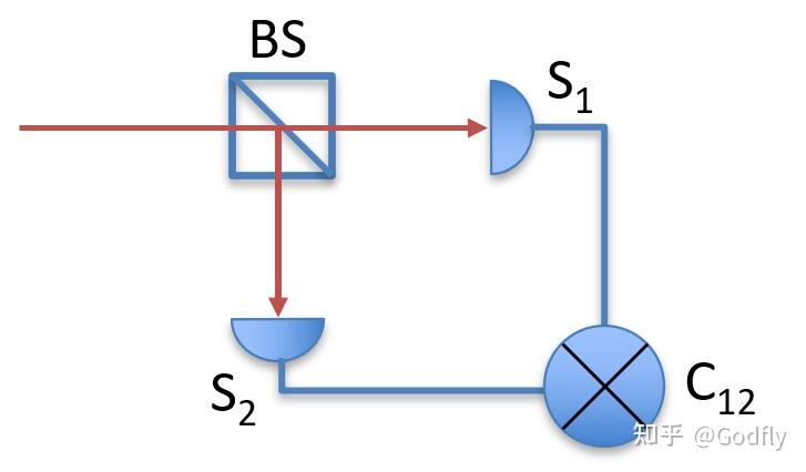
Anyone doing quantum optics experiments certainly knows that the HBT experiment can be used to measure the second-order correlation function g2. That is, a beam of light is split into two beams using a 50:50 beam splitter, which are then detected by two separate detectors, and the variation of the correlation between the intensities on the two sides with delay is counted, as shown below:

Hanbury Brown and Twiss Experiment

Generalized Quantum Measurements: An Introduction to POVMs

Projective Measurements

A measurement in the traditional sense (in the Von Neumann sense) is a collection of projection operators. By performing a spectral decomposition of the self-adjoint operator corresponding to an observable \(O=\sum_i\lambda_i |\varphi_i\rangle\langle\varphi_i|\) , one obtains these projection operators \(|\varphi_i\rangle\langle\varphi_i|\) . Anyone who has studied elementary quantum mechanics should be familiar with this part.

In addition to Von Neumann measurements, there is a more general type of measurement called a generalized measurement (Generalized Measurements), also known as a POVM (Positive Operator Valued Measure).

Distinguishing Mixed States from Entangled States

I. Pure States and Mixed States

To understand pure states and mixed states, one must first understand the density operator, or density matrix.

1.1 What Is a Density Operator?

When I first encountered the density operator, I found it quite remarkable. This is because it takes the tensor product of a state with its own dual:

\[v \mapsto v\otimes v^*\]

Or, written in a more physics-style manner:

\[| \psi \rangle \mapsto |\psi \rangle \langle \psi |\]

We all know that a quantum state \(v\) is merely a vector in a Hilbert space, namely \(v \in H\) . But why insist on making the density operator \(v\otimes v^*\in H\otimes H^* \cong \operatorname{End}(H)\) ? What is the point of this?

What is the relationship between Lie derivative and covariant derivative?

I. Differences and Similarities in Properties

Lie derivative $\mathcal{L}_V$ and covariant derivative $\nabla_V$ share many common points:

  1. Both $\mathcal{L}_V$ and $\nabla_V$ preserve the type of tensors, mapping $\mathcal{T}^p_q(M)$ to $\mathcal{T}^p_q(M)$. $\mathcal{T}^p_q(M)$ represents the set of all smooth tensor fields of type (p, q) on $M$.

Particularly, for (0,0) type tensor fields, i.e., scalar fields $f\in \mathcal{F}(M)$, we have $\mathcal{L}_V f=\nabla_V f=Vf$.

  1. Both satisfy linearity and the Leibniz rule:

$ \begin{aligned} \mathcal{L}_V(\mu A + \lambda B) &= \mu \mathcal{L}_V A + \lambda \mathcal{L}_V B, \\ \mathcal{L}_V (A \otimes B) &= (\mathcal{L}_V A)\otimes B + A \otimes (\mathcal{L}_V B) \end{aligned} $