1 Basics

SPI has three-wire mode and four-wire mode. The three-wire mode consists of three wires - SS (Slave Select), SCK (SPI Clock), and MOSI (Master-In-Slave-Out). The four wire mode has an extra line called MISO (Master-In-Slave-Out).

SPI clock has four modes: CPOL=0/1 and CPHA=0/1. CPOL stands for clock polarity – clock low or high when in idle. CPHA stands for clock phase – data valid at 0 degree or 180 degrees.

Let’s look at a code snippet in the Jupyter Notebook:

 1
 2
 3
 4
 5
 6
 7
 8
 9
10

import time
import ipywidgets as widgets
from IPython.display import display

slider = widgets.IntSlider()
display(slider)

while True:
    print(slider.value)
    time.sleep(1)

IntSlider is an interactive Jupyter Notebook widget. When the user interacts with the slider, the slider value should change.

However, if you run the above codes, you will find that the printed value of the slider won’t change at all – it will be stuck at its initial value.

Recently, I have been using Python coroutines/asynchronous programming in a project. Now, I will summarize my experience.

Import

1

import asyncio

If asyncio is to be used in an IPython environment, we have to add two more lines：

1
2
3

import nest_asyncio
nest_asyncio.apply()
import asyncio

Coroutines

Coroutines are the core of asynchronous programming in Python. To define a coroutine, you need to use async def.

1
2
3

async def main():
    # do something
    print("Hello world!")

To execute the coroutine, you cannot directly call main(). Instead, you need to use run():

Windows

Set a network adapter that can access the internet in the Control Panel and share it with Ethernet. The IP address of Ethernet will change to 192.168.137.1 (this is the default behavior in Windows).

Then, set the gateway as 192.168.137.1 in the terminal of the development board:

sudo route add default gw 192.168.137.1

Set the IP address as 192.168.137.x, where x is any value except 1 and 255 (gateway address and broadcast address):

Xilinx’s toolchain consumes soooo much memory! Sometimes it causes the system to freeze… After all, my laptop only has 8GB of RAM. So there’s no other choice but to add virtual memories.

After increase the swapfile, the system performance has improved a lot:

1
2
3
4

sudo swapoff /swapfile
sudo dd if=/dev/zero of=/swapfile bs=1M count=16384
sudo mkswap /swapfile
sudo swapon /swapfile

To partition and format an SD card in Linux, follow these steps: First, connect the SD card to your PC. Then, use the fdisk command in the bash command line to partition the SD card. Finally, use the mkfs command to create a file system (format) on the SD card.

The main commands are as follows:

First, use sudo fdisk -l to confirm which device in /dev corresponds to the SD card.

To mount the EFI partitions, run the following commands in PowerShell:

1
2
3
4
5
6

diskpart
list disk  # make sure which is the disk that contains the EFI partition. usually 0
select disk 0
list partition # make sure which is the EFI partition. normally 0
select disk 0
assign letter=z

Then we will mount the EFI partition as drive Z.

This operation may be useful when using a dual-boot system with Windows and Ubuntu: Sometimes, after removing the Ubuntu system, only the Windows system remains, but the GRUB interface still appears every time the computer boots. In this case, you need to delete the old Ubuntu EFI partition.

I recently discovered this fantastic tool for creating personal websites - Hugo. Feels really cool and user-friendly! Plan to gradually migrate my blogs from Zhihu to here in the future.

Differential Forms

Before introducing curl, we must first introduce differential forms and the exterior derivative operator.

An n-form can be defined as an alternating multilinear map \(\omega:(T_pM)^n\rightarrow \mathbb{R}\) . It maps multiple vectors to a real number. Moreover, it satisfies alternation: exchanging two input vectors introduces an additional minus sign in the output.

Thus, an n-form can be explicitly defined as follows:

The set of all n-forms on \(T_pM\) can be written as \(\bigwedge^n(T^*_pM)\) .

In physics books, we often encounter the terms “pseudovector” (pseudo-vector) and “pseudoscalar” (pseudo-scalar).

In fact, on a 3-dimensional manifold, a “pseudovector” is the exterior product of two tangent vectors \(v\in T_pM\wedge T_pM=\bigwedge^2(T_pM)\), while a “pseudoscalar” is the exterior product of three tangent vectors \(s\in T_pM\wedge T_pM\wedge T_pM=\bigwedge^3(T_pM)\).

After equipping the space with an inner product (or a nondegenerate bilinear form), there is a Hodge duality relation between \(\bigwedge^2(T_pM)\) and \(\bigwedge^1(T_pM)\), so we “mistakenly regard” pseudovectors as vectors. Similarly, because there is a Hodge duality relation between \(\bigwedge^3(T_pM)\) and \(\bigwedge^0(T_pM)\) (a scalar field), we “mistakenly regard” pseudoscalars as scalars.

Preface

As a physics student, you have probably heard of one or more of the concepts tensor, differential form, exterior algebra, connection/curvature, and so on. But, like me, you may feel completely lost whenever you hear these concepts. This article therefore aims to help physics students organize these closely interconnected ideas.

The structure of this article is as follows:

a. In Chapter 1, we introduce the stage on which physics takes place: differentiable manifolds, and define scalar fields on manifolds.

There are two cases to consider: physical addresses and virtual addresses.

If we are talking about physical address 0x0, then it is not lonely at all. Every time the system resets, the program counter stops by to say hello:

“Hey, buddy, how do I get to the reset interrupt service routine?”

“Go to 0x100000!”

“Thanks!”

This is because, on most architectures, the interrupt vector table is placed at physical address 0x0. And the first interrupt is the reset interrupt.

0. Introduction to the Problem

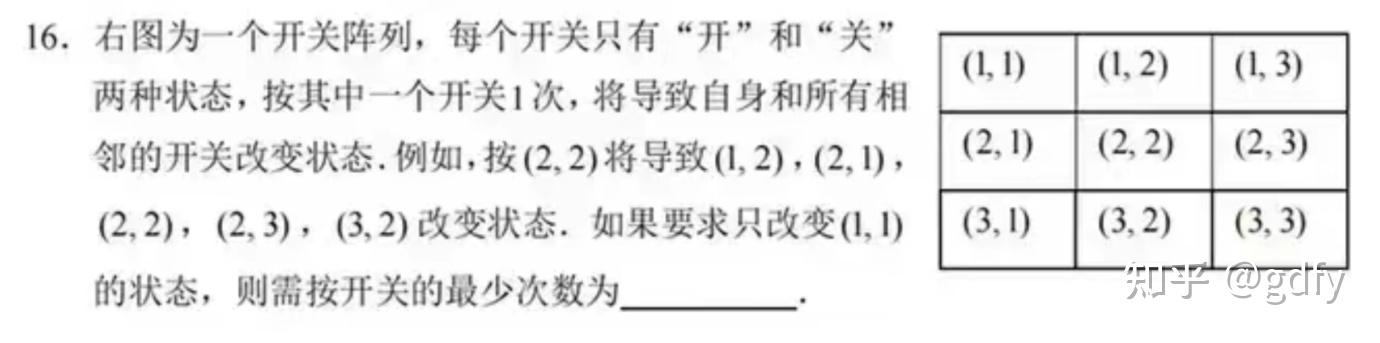
With this single college entrance examination mock question, we can review concepts from abstract algebra such as groups, rings, fields, modules, and vector spaces. The problem is shown below:

A college entrance examination mock question from somewhere; in fact, you can figure it out with a little trial and error—it is not difficult.

Simply put, it is a matter of “pulling one hair and moving the surrounding area.” Changing one cell also rotates the surrounding cells. I believe many people have played this puzzle game. Even elementary school students can understand this game.

Introduction

When I first began studying physics, I was somewhat confused about the concepts of wave packets and group velocity. Looking back now, they are actually very simple; it is just that some textbooks do not explain them clearly. This article reviews the concept of group velocity and several examples of dispersion relations.

Momentum Eigenstates and Fourier Transforms

The wave function of a plane wave

cannot be normalized.

According to the postulates of quantum mechanics, all physically existing wave functions are normalizable. Therefore, momentum eigenstates \(|p\rangle\) do not represent physically existing states. In other words, momentum cannot be measured with complete precision.

The following formulas can make problem solving much more convenient.

I. Gaussian Integrals

Here is a convenient way to remember it:

First, remember

Next,

This formula applies to both odd and even cases of \(n\).

If you are dealing with Gaussian functions (for example, in probability theory), then this integral will appear very frequently!

II. Powers of Trigonometric Functions

The following expression gives \(I_n\)

I believe that anyone learning vector calculus for the first time finds the product rules for vectors quite daunting:

Easy difficulty:

Hard difficulty:

Hell difficulty:

DLC: second derivatives

A Concise Proof

To make the proof as concise as possible, we would like to use a single expression with subscripts to represent multiple expressions, rather than having to write out x, y, and z every time.

You do not need to know any formulas to gain an intuitive understanding of various phenomena in special relativity (length contraction, time dilation, the twin paradox, etc.).

A Small Modification to the Galilean Transformation

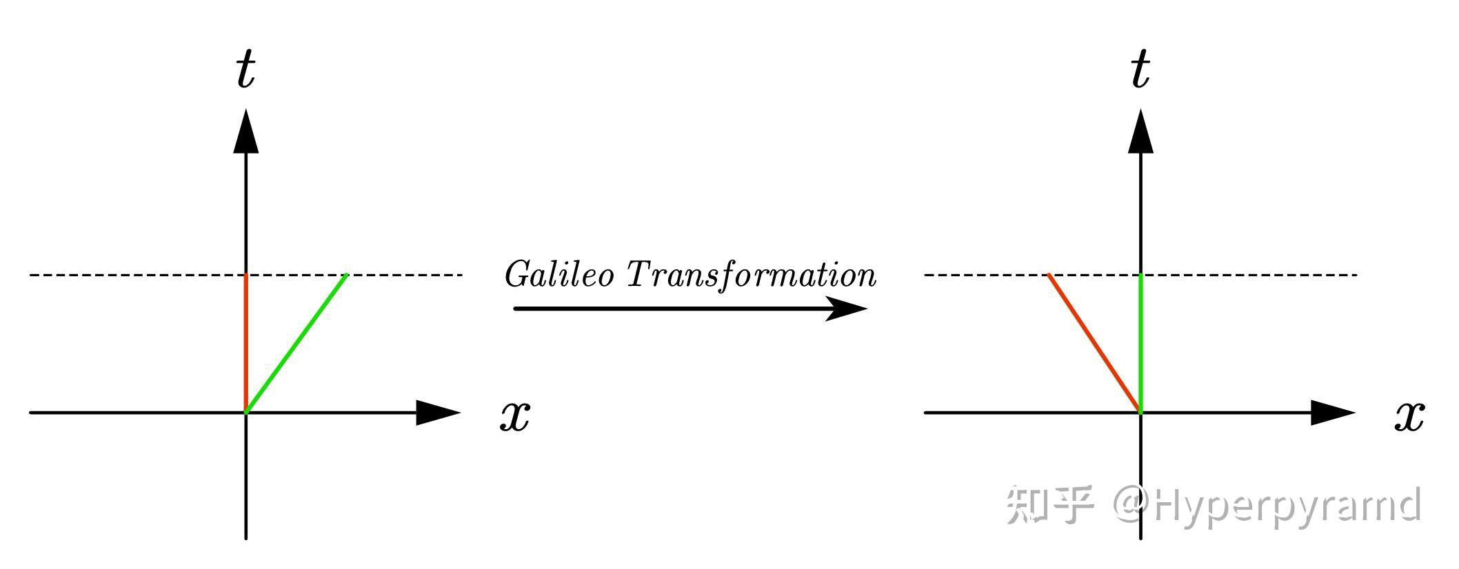
Let us first look at the classical Galilean transformation. In a t-x diagram, the Galilean transformation appears as a shear transformation. Points slide along lines parallel to the x-axis.

Galilean transformation, viewed from Little Red’s and Little Green’s perspectives

Link to the Previous Article

Foundations of Axiomatic Set Theory (Part I): The Empty Set and Russell’s Paradox## Constructing Natural Numbers (ZF3: Axiom of Pairing, ZF4: Axiom of Union)

In the previous article, we successfully defined a unique set called the empty set and resolved Russell’s paradox. Next, we will use the empty set to construct more sets. To do so, we need more constructive axioms.

Axiom of Pairing: \(\forall a \forall b \exists c \forall x((x\in c)\leftrightarrow (x=a )\vee (x=b))\)

21/03/2025: Major revision of this article

What Is the Invariance of Differential Forms?

According to textbooks, the invariance of differential forms means that, under a change of variables, the form of a differential equation remains unchanged. That is:

If, when \(\mathrm{d}y\) in \(y\) denotes the function \(y=f(x)\) and \(\mathrm{d}x\) in \(x\) denotes the function \(\phi(x)=x\), \(\mathrm{d}y=a\mathrm{d}x\) holds, that is, \(\mathrm{d}f=a\mathrm{d}\phi\) holds,

then, when \(\mathrm{d}y\) in \(y\) denotes the function \(y=g(t)\) and \(\mathrm{d}x\) in \(x\) denotes the function \(x=\varphi(t)\), \(\mathrm{d}y=a\mathrm{d}x\) likewise holds, that is, \(\mathrm{d}g=a\mathrm{d}\varphi\) holds.

I. Is a Differential an Infinitesimal?

Physicists like to regard a differential as a very small quantity. This is always convenient in calculations, but it gives one a feeling of imprecision.

In fact, it is indeed imprecise; the second mathematical crisis arose for this reason.

Rigor and accessibility are forever complementary. Regarding a differential as an infinitesimal caters to intuitive sensibilities, yet cannot pass rational scrutiny.

II. A Differential Is a Linear Function

I prefer to think of a differential (at a certain point) as a machine. For example,