Stop Being Looked Down Upon by Math Majors! What Physicists Need to Know About Uniform Convergence When Interchanging Operations
 Haifei
Preface
Whenever physicists perform operations such as differentiating under the integral sign or interchanging the order of integration, the mathematicians watching can no longer sit still:
“Does your improper integral/series converge uniformly?”
The physicist replies:
“What is uniform convergence? We have always done it this way.”
Or:
“Assume that this function has sufficiently nice properties.”
Or, even more outrageously:
“Assume that this function looks rather pretty.”
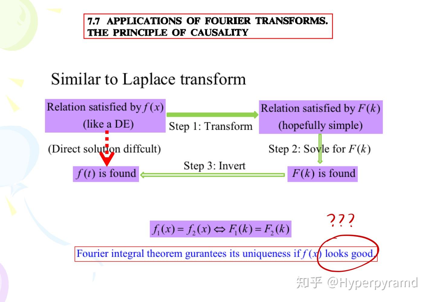
looks good
…
So the mathematician leaves, grumbling…

Image source: the Internet; please contact us for removal if infringing
However, as physicists, there is no harm in learning about these mathematically rigorous conditions.
This article aims to clarify the commonly used “dangerous operations” in physics related to uniform convergence.
At a Glance
Uniform convergence guarantees the legitimacy of interchanging operations, including:
- Interchanging an infinite summation sign and a limit sign
- Interchanging an infinite summation sign and a differentiation sign
- Interchanging an infinite summation sign and an integration sign
- Interchanging an improper integral sign and a limit sign
- Interchanging an improper integral sign and a differentiation sign
- Interchanging an improper integral sign and an integration sign
I. Series of Functions
We all know that:
The sum of two continuous functions is still continuous.
The sum of the derivatives of two functions is no different from the derivative of their sum.
The sum of the Riemann integrals of two functions over an interval should equal the Riemann integral of their sum.
This is due to the linearity of limits, derivatives, and integrals.
But what if we are adding not two functions, but infinitely many functions?
The sum of infinitely many functions is called a series of functions.
Series of functions such as Taylor series and Fourier series all involve sums of infinitely many functions.
Experience shows that a sum with infinitely many terms differs greatly from one with finitely many terms. If handled carelessly, it may lead to some absurd conclusions.
1.1 Uniform Convergence of Series of Functions
So, what must we pay attention to in order to extend the three properties above (term-by-term addition, term-by-term differentiation, and term-by-term integration) to sums of infinitely many functions?
That is right: uniform convergence.
Definition 1.1 (Uniform Convergence of a Series of Functions)
Let \(S_n(x)\) be the partial sum of a series of functions. Then, a series satisfying \(\lim_{n\rightarrow \infty} \sup_{x\in D}|S_n(x)-S(x)|=0\) is said to converge uniformly to \(S(x)\) on \(D\) .
In plain language, if the absolute value of the difference between the partial sum function and \(S(x)\) (which is itself also a function) has a controllable upper bound (one independent of the independent variable \(x\)), then the partial sum functions converge uniformly to \(S(x)\).
This definition also applies to ordinary sequences of functions; one need only replace \(S_n(x)\) with the general term of the sequence of functions.
Example 1.1
\[ S(x)= \begin{cases} 0&0\le x\lt 1\\ 1&x=1 \end{cases} \]
To show the reader that uniform convergence is stronger than ordinary pointwise convergence, let us give a simple example. Let the partial sum function (or the general term of a sequence of functions) be \(S_n(x)=x^n\). Clearly, on the interval \([0,1]\), it converges pointwise to the function.
However, no matter how large \(n\) is, the partial sum function \(S_n(x)\) can always attain the value \(0.5\) (by the continuity of the partial sum function and the intermediate value theorem). In other words, \(\forall n\exists x_0(S_n(x_0)=0.5)\). This makes it impossible to control the upper bound: there are always some \(x\) that you cannot control. In fact, in this example, no matter how large \(n\) is, the supremum of the error (that is, the \(\sup\) symbol) is always \(1\).
Uniform convergence, on the other hand, allows one to control all \(f(x)\) simultaneously, making them all approach the target function arbitrarily closely according to the desired upper bound \(\epsilon\).
Example 1.2
Let us give another simple example.
Suppose we come up with a very foolish idea: using \(y=\mathrm{e}^{\alpha x}\,(\alpha\rightarrow0)\) to approximate \(y=1\).
We can then consider the sequence of functions \(\varphi_k(x)=\mathrm{e}^{\frac{1}{k}x}\). Clearly, \(\lim_{k\rightarrow \infty}\mathrm{e}^{\frac{1}{k}x}=1\) holds for all \(x\).
However, as long as \(\frac{1}{k}\ne 0\), \(\varphi_k(x)=\mathrm{e}^{\frac{1}{k}x}\) is unbounded on \(\mathbb{R}\).
Suppose your boss sets a target \(\epsilon\) for you and orders you to find an \(N\) such that, when \(k\gt N\), the error \(\left|\mathrm{e}^{\frac{1}{k}x}-1\right|\lt \epsilon\) holds for all \(x\). You may want to consider resigning, because this is clearly an impossible task. No matter how large an \(N\) you find, there will certainly be a larger \(x\) that ruins the plan. Suppose that for the case of \(\epsilon =1\), you have found an \(N\) satisfying the requirements; then your boss need only set \(x=2N\), and we have \(\left|\mathrm{e}^{\frac{1}{k}2N}-1\right|\gt \mathrm{e}-1\gt 1\quad (N\lt k\lt 2N)\).
1.2 Series of Functions: Uniform Convergence and Interchanging Operations
Let us now see what it means to interchange operations.
Theorem 1.1 (Continuity, Differentiability, and Integrability of a Series of Functions)
If the series \(\sum_{k}f_k(x)\) converges uniformly, then
(a) If every term of the series is continuous, then the sum of the series is continuous. In other words, the summation sign may be interchanged with the limit sign:
\(\lim_{x\rightarrow x_0}\sum_{k} f_k(x)=\sum_{k} \lim_{x\rightarrow x_0} f_k(x)\) .(b) If the derivative of every term of the series is continuous, and the series formed by the derivatives converges uniformly, then the series may be differentiated term by term. In other words, the summation sign may be interchanged with the differentiation sign:
\(\frac{\mathrm{d}}{\mathrm{d}x}\sum_{k} f_k(x)=\sum_{k} \frac{\mathrm{d}}{\mathrm{d}x} f_k(x) \) .(c) If every term of the series is continuous, then the series may be integrated term by term. In other words, the summation sign may be interchanged with the integration sign:
\(\int_{M}\sum_{k} f_k(x) \mathrm{d}x=\sum_{k} \int_{M}f_k(x) \mathrm{d}x\) (the subscript M denotes the definite integral over the interval M).
As can be seen, the various interchanges beloved by physicists can have their legitimacy guaranteed by uniform convergence.
Note: In Theorem 1.1(b), note that the series formed by the derivatives is required to converge uniformly.
In addition, in Theorem 1.1(b), if the original series converges, then uniform convergence of the series of derivatives together with continuity of each derivative implies uniform convergence of the original series.
Example 1.3
Returning to the previous example \(S(x)=x^1+(x^2-x^1)+(x^3-x^2)+\cdots= \begin{cases} 0&0\le x\lt 1\\ 1&x=1 \end{cases}\). Every term of this series is continuous, but its sum is not continuous, so it does not converge uniformly.
In fact, Theorems 1.1(b) and 1.1(c) are direct consequences of the following theorem:
If \(\{\varphi_k(x)\}\) converges uniformly to \(f(x)\), and for every \(k\), \(\varphi_k{(x)}\) is continuous, then: \(\frac{\mathrm{d}}{\mathrm{d}x}f(x)=\frac{\mathrm{d}}{\mathrm{d}x}\lim_{k\rightarrow \infty} \varphi_k(x)=\lim_{k\rightarrow \infty} \frac{\mathrm{d}}{\mathrm{d}x} \varphi_k(x) \), as well as \(\int_{M}f(x){\mathrm{d}x}=\int_{M}\lim_{k\rightarrow \infty} \varphi_k(x){\mathrm{d}x}=\lim_{k\rightarrow \infty} \int_{M} \varphi_k(x) {\mathrm{d}x}\)
One need only replace the general term \(\varphi_k(x)\) in this theorem with the partial sum \(S_k(x)\). Thus, we have also mastered the interchange of the limit sign with the differentiation sign, and the interchange of the limit sign with the integration sign. Since sequences of functions usually appear in physics in the form of partial sums, these two interchanges are not often used.
It is worth mentioning that the “summation sign” in the interchanges above refers to infinite summation. If one is summing only finitely many terms, it is not a series at all, so there is no question of convergence. Of course, interchanging finite sums is very safe; one can simply interchange them directly.
II. Improper Integrals with Parameters
2.1 Integrals with Parameters
When finding the sum of a series, we can think of it this way: each term in a series of functions originally depends on both the index and the independent variable, namely
\[\varphi(x;k)=\varphi_k(x)\]Then, summing over \(k\) makes the letter \(k\) disappear:
\[\sum_{k}\varphi_k(x)=S(x)\]Only \(x\) remains.
Similarly, we can do the same with an integral. Suppose that some quantity depends on two variables: \(y=\varphi(x,s)\)
Now, instead of summing over \(s\), we integrate over \(s\):
\[\int_{a}^{b}\varphi(x,s)\mathrm{d}s=f(x)\]This makes \(s\) disappear, leaving only \(x\).
This is an integral with a parameter. Here \(x\) is the parameter; choosing different \(x\) can give the integral different values.
Example 4
Observe \(\int_{0}^{+\infty}\mathrm{e}^{-x}\mathrm{d}x=1\), \(\int_{0}^{+\infty}\mathrm{e}^{-2x}\mathrm{d}x=\frac{1}{2}\), \(\int_{0}^{+\infty}\mathrm{e}^{-3x}\mathrm{d}x=\frac{1}{3}\), …
It can be seen that \(\int_{0}^{+\infty}\mathrm{e}^{-kx}\mathrm{d}x\) should have a functional relationship with \(k\). In fact, this relationship is \(\int_{0}^{+\infty}\mathrm{e}^{-kx}\mathrm{d}x=\frac{1}{k}\quad (k\gt 0)\), and it is easy to prove.
Here, \(k\) is the “parameter” of the integral with a parameter.
2.2 Integrals with Parameters: Interchanging Operations
What interests us is what properties an integral with a parameter has with respect to the parameter. For example, is it continuous in the parameter? That is, is \(\int_{a}^{b}\varphi(x,s)\mathrm{d}s=f(x)\) continuous?
There are also more interesting questions, such as whether it can be differentiated under the integral sign.
Example 5
Differentiating both sides of \(\int_{0}^{+\infty}\mathrm{e}^{-kx}\mathrm{d}x=\frac{1}{k}\quad (k\gt 0)\) gives \(\frac{\mathrm{d}}{\mathrm{d}k}\int_{0}^{+\infty}\mathrm{e}^{-kx}\mathrm{d}x=-\frac{1}{k^2}\quad (k\gt 0)\)
It is not hard to find that putting the differentiation inside the integral sign also gives the correct result: \(\int_{0}^{+\infty}\frac{\partial}{\partial k}\mathrm{e}^{-kx}\mathrm{d}x=-\frac{1}{k^2}\quad (k\gt 0)\)
When is this operation permitted? The following theorem answers this question:
Theorem 2.1 (Continuity, Differentiability, and Integrability of Riemann Integrals with Parameters)
\(I(y)=\int_{\alpha}f(x,y)\mathrm{d}x, \, x\in \alpha, \, y \in \beta\), \(\alpha\), and \(\beta\) are bounded closed intervals.
(a) If \(f\) is continuous on \(\alpha \times \beta\), then \(I(y)\) is continuous on \(\beta\). In other words, the limit sign and the integral sign may be interchanged.
(b) If \(f\) and \(\frac{\partial f}{\partial y}\) are continuous on \(\alpha \times \beta\), then \(I(y)\) is differentiable on \(\beta\), and \(\frac{\mathrm{d}}{\mathrm{d}y}I(y)=\int_{\alpha}\frac{\partial}{\partial y}f(x,y)\mathrm{d}y\). In other words, differentiation and integration may be interchanged.
(c) If \(f\) is continuous on \(\alpha \times \beta\), then \(I(y)\) is integrable on \(\beta\), and \(\int_{\beta}\mathrm{d}y\int_{\alpha}f(x,y)\mathrm{d}x=\int_{\alpha}\mathrm{d}x\int_{\beta}f(x,y)\mathrm{d}y\). In other words, the integration signs may be interchanged.
The reader may wonder: there is no uniform convergence here? Of course not. An integral over a closed interval is always bounded; it cannot diverge at all, so there is no concept of convergence, much less uniform convergence. However, improper integrals do not necessarily converge. Let us now look at improper integrals.
2.3 Improper Integrals with Parameters
Put simply, improper integrals are integrals over unbounded intervals or bounded open intervals. They may fail to converge!
The convergence of the improper integral \(\int_{a}^{+\infty}f(x)\mathrm{d}x\) over an unbounded interval is defined as follows: for every \(\epsilon\gt 0\), there exists \(N\) such that when \(M\gt N\), \(\left|\int_{M}^{+\infty}f(x)\mathrm{d}x\right|\lt \epsilon\).
2.4 Improper Integrals with Parameters: Uniform Convergence and Interchanging Operations
If we add another parameter \(f(x;y)\) to \(f(x)\) (the parameter has changed to \(y\) here; hopefully you are not confused), the same question arises: for all different parameter values \(y\), can we use a single \(N\) to control the error? This is the question of uniform convergence for improper integrals.
Definition 2 (Uniform Convergence of Improper Integrals with Parameters)
If, for every \(\epsilon\gt 0\), there exists \(N(\epsilon)\) such that when \(M\gt N(\epsilon)\), \(\left|\int_{M}^{+\infty}f(x,y)\mathrm{d}x\right|\lt \epsilon\), then the improper integral \(\int_{a}^{+\infty}f(x,y)\mathrm{d}x\) is said to converge uniformly.
(Or \(\lim_{M\rightarrow \infty} \sup_{y\in \beta}\left|\int_{M}^{+\infty}f(x,y)\mathrm{d}x\right|=0\))
Clearly, if an improper integral converges uniformly, then because \(N(\epsilon)\) is independent of \(y\), for any given upper bound \(\epsilon\), we can use only one \(N(\epsilon)\) to control all \(y\) at once, without needing to tailor a set of \(N(\epsilon,y)\) for every \(y\). This is similar to the case of series of functions discussed above.
For other types of improper integrals, such as improper integrals over bounded open intervals, the method of discussion is similar and will not be repeated.
The relevant theorems for improper integrals with parameters require only that we add the condition of uniform convergence to the theorems for Riemann integrals with parameters (Theorem 2.1).
Theorem 2.3 (Continuity, Differentiability, and Integrability of Improper Integrals with Parameters)
Given the improper integral \(I(y)=\int_{\alpha}f(x,y)\mathrm{d}x, \, x\in \alpha, \, y \in \beta\), \(\beta\) is a bounded closed interval, and \(I(y)\) converges uniformly.
a) If \(f\) is continuous on \(\alpha \times \beta\), then \(I(y)\) is continuous on \(\beta\). In other words, the limit sign and the integral sign may be interchanged.
b) If \(f\) and \(\frac{\partial f}{\partial y}\) are continuous on \(\alpha \times \beta\), and \(\int_{\alpha}\frac{\partial f}{\partial y}(x,y)\mathrm{d}x\) converges uniformly, then \(I(y)\) is differentiable on \(\beta\), and \(\frac{\mathrm{d}}{\mathrm{d}y}I(y)=\int_{\alpha}\frac{\partial}{\partial y}f(x,y)\mathrm{d}y\). In other words, differentiation and integration may be interchanged.
c) If \(f\) is continuous on \(\alpha \times \beta\), then \(I(y)\) is integrable on \(\beta\), and \(\int_{\beta}\mathrm{d}y\int_{\alpha}f(x,y)\mathrm{d}x=\int_{\alpha}\mathrm{d}x\int_{\beta}f(x,y)\mathrm{d}y\). In other words, the integration signs may be interchanged.
Therefore, for ordinary Riemann integrals, continuity alone is sufficient for various interchanges; uniform convergence is not needed (nor is there a concept of uniform convergence, just as finite sums of functions do not require convergence). But for improper integrals, interchanging operations still requires uniform convergence.
Summary
Two kinds of uniform convergence were discussed above: one is the uniform convergence of series of functions, and the other is the uniform convergence of improper integrals with parameters.
According to Theorem 1.1, uniform convergence of a series of functions guarantees the legitimacy of the following operations:
Interchanging an infinite summation sign and a limit sign,
Interchanging an infinite summation sign and a differentiation sign,
Interchanging an infinite summation sign and an integration sign.
According to Theorem 2.2, uniform convergence of an improper integral with parameters guarantees the legitimacy of the following operations:
Interchanging an improper integral sign and a limit sign,
Interchanging an improper integral sign and a differentiation sign,
Interchanging an improper integral sign and an integration sign.
When interchanging with the differentiation sign, note that not only the original series but also the series of derivatives must converge uniformly.