Wave Packets, Group Velocity, and Dispersion Relations

Introduction

When I first began studying physics, I was somewhat confused about the concepts of wave packets and group velocity. Looking back now, they are actually very simple; it is just that some textbooks do not explain them clearly. This article reviews the concept of group velocity and several examples of dispersion relations.

Momentum Eigenstates and Fourier Transforms

The wave function of a plane wave

\[|\bm p\rangle=\frac{1}{(2\pi\hbar)^{3/2}}\exp(\mathrm{i}\frac{\bm{p}}{\hbar}\cdot\bm{x})\]

cannot be normalized.

According to the postulates of quantum mechanics, all physically existing wave functions are normalizable. Therefore, momentum eigenstates \(|p\rangle\) do not represent physically existing states. In other words, momentum cannot be measured with complete precision.

Suppose that momentum could be measured precisely. Then after the measurement, the system would collapse into an eigenstate of the momentum operator, but such an eigenstate cannot exist in reality; therefore, momentum cannot be measured precisely.

However, plane waves, as abstract mathematical entities, are very useful for analysis. That is, we can decompose a physically existing wave into a superposition of monochromatic waves:

\[|\psi\rangle=\sum_{\bm p}\langle \bm p|\psi \rangle |\bm p\rangle=\int\langle \bm p|\psi \rangle |\bm p\rangle\mathrm{d}^3\bm p\]

This is in fact the Fourier transform.

The above relation can also be expressed using wave vectors:

\[|\bm k\rangle=\frac{1}{(2\pi)^{3/2}}\exp(\mathrm{i}\bm{k}\cdot \bm{x})\]\[|\psi\rangle=\sum_{\bm k}\langle \bm k|\psi \rangle |\bm k\rangle=\int\langle \bm k|\psi \rangle |\bm k\rangle\mathrm{d}^3\bm k\]

The above procedure applies not only to wave functions in quantum mechanics, but to all square-integrable functions.

---

Group Velocity and Phase Velocity

Most physically existing wave functions are localized, meaning that most of their energy is confined to a certain region; this is a wave packet.

The velocity at which a wave packet moves is called the group velocity. It is a first-order approximation to the motion of a wave packet:

\(\bm v_g=\nabla_{\bm k}\omega(\bm k)\) （*）

The counterpart of group velocity is phase velocity, defined as

\[\bm v_p=\frac{\omega}{k}\hat{\bm k}\]

The reason group velocity is said to be only an approximation to wave-packet motion is that a wave packet does not necessarily retain its shape as it propagates. In other words, group velocity alone cannot fully describe the evolution of a wave packet.

In fact, because the components of different monochromatic waves in a wave packet have different phase velocities, the wave packet spreads out as it propagates. If the wave packet spreads too much, the definition of group velocity becomes ill-posed.

The condition for a wave packet to retain its shape is that the phase velocities of different monochromatic waves have the same magnitude, namely \(\omega=Ck\), with \(C\) constant. In this case, the group velocity equals the phase velocity.

It can be seen from equation （*） that the group velocity depends on the form of \(\omega(\bm k)\). \(\omega(\bm k)\) is the so-called dispersion relation.

Example 1 For electrons in free space, \(\omega=\frac{\hbar k^2}{2m}\) and \(\bm v_g=\frac{\hbar \bm k}{m}\). The phase velocity is \(\bm v_p=\frac{\hbar \bm k}{2m}\). Thus, for an electron wave packet in free space, its group velocity is twice its phase velocity.

For electrons in a lattice, the situation is more complicated due to the presence of a periodic potential. In this case, \(\omega(k)\) no longer varies quadratically, but instead behaves as shown in the figure below:

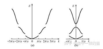
Note that energy is proportional to frequency.

It can be seen that at the boundary of the Brillouin zone, the dispersion relation is discontinuous, and thus a “band gap” is formed.

The existence of band gaps is the foundation of semiconductor physics. The switching of transistors in computers is, in fact, achieved by using voltage to control the position of the Fermi level within the band gap, thereby controlling the electron concentration in the conduction band.

The concepts of phase velocity and group velocity apply not only to wave functions, but to all waves.

Example 2 For electromagnetic waves in vacuum, \(\omega=ck\), so their phase velocity and group velocity are both equal to the speed of light in vacuum, namely \(v_p=v_g=c\).

For electromagnetic waves in a medium, the situation is more complicated. Since the refractive index \(n\) is not \(1\) and depends on \(\omega\), we have \(\omega=\frac{c}{n(\omega)}k\), \(\bm v_p=\frac{c}{n(\omega)}\), and hence
\(\begin{aligned} \nabla_{\bm k}\omega&=\nabla_{\bm k}(v_p k)=\bm v_p+k\nabla_{\bm k}v_p\\&=\bm v_p-k\frac{c}{[n(\omega)]^2}\frac{\mathrm{d} n(\omega)}{\mathrm{d} \omega}\nabla_{\bm k}\omega\\ &=\bm v_p-k\frac{v_p}{n(\omega)}\frac{\mathrm{d} n(\omega)}{\mathrm{d} \omega}\nabla_{\bm k}\omega \end{aligned}\)
Thus \(\bm v_g=\nabla_{\bm k}\omega=\frac{\bm v_p}{1+k\frac{v_p}{n}\frac{\mathrm{d}n}{\mathrm{d}\omega}}\)

In the normal-dispersion region, \(\frac{\mathrm{d}n}{\mathrm{d}\omega}\gt 0\), and the group velocity \(v_g\) is less than the phase velocity \(v_p\), which is less than the speed of light. In the anomalous-dispersion region, \(\frac{\mathrm{d}n}{\mathrm{d}\omega}\lt 0\), and the group velocity is greater than the phase velocity and can even exceed the speed of light. However, in the anomalous-dispersion region, the phase velocities of monochromatic light of different wavelengths differ greatly, so the wave packet quickly spreads out, and the definition of group velocity becomes ill-posed.

Some popular-science accounts say that group velocity is the velocity of energy propagation. This is incorrect. Remember that group velocity is only a first-order approximation to wave-packet motion and cannot fully describe the evolution of a wave packet. A group velocity exceeding the speed of light does not imply that energy/information travels faster than light; rather, in this situation, group velocity has already lost its meaning.

Example 3 In a phonon dispersion curve, the branch passing through the origin is called the acoustic branch. In the long-wavelength limit (that is, \(k\rightarrow0\)), \(\omega(k)\) is approximately linear, \(\omega(k)=v_sk\), and the group velocity then equals the phase velocity and the speed of sound, namely \(v_p=v_g=v_s\).

For the optical branch in the long-wavelength limit, \(\mathrm{d}\omega/\mathrm{d}k=0\). The group velocity is then zero, corresponding to a standing wave, while the phase velocity tends to infinity.

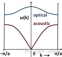
Phonon dispersion relation of a one-dimensional diatomic chain

As can be seen from the examples above, both phase velocity and group velocity can exceed the speed of light.

Derivation of the Group Velocity Formula

So where does equation （*） come from? Why is group velocity the gradient of angular frequency with respect to wave vector? Let us derive it for the one-dimensional case below.

First, a wave packet can be decomposed into a superposition of plane waves:

\[f(x,t)=\frac{1}{2\pi}\int_{-\infty}^{\infty}F(k)\exp[\mathrm{i}(kx-\omega t)]\mathrm{d}k\]

This is the Fourier integral (or Fourier transform).

Now consider a wave packet whose plane-wave components \(F(k)\) are distributed over a relatively small range; otherwise, it will quickly spread out. That is, \(F(k)\) is nonzero only near \(k=k_0\).

Therefore, the dispersion relation can be approximated as:

\[\omega(k)\approx \omega(k_0)+\left.\frac{\mathrm{d}\omega}{\mathrm{d}k}\right|_{k=k_0}\cdot(k-k_0)\]

Let us simplify the notation:

\[\omega=\omega_0+\omega_0^{\prime}\cdot \widetilde{k}\]

where

\(\omega_0=\omega(k_0)\), \(\omega^\prime=\left.\frac{\mathrm{d}\omega}{\mathrm{d}k}\right|_{k=k_0}\), \(\widetilde{k}=k-k_0\).

Substituting into the Fourier integral gives:

\[\begin{aligned} f(x,t)&=\frac{1}{2\pi}\int_{-\infty}^{\infty}F(k)\exp[\mathrm{i}(kx-\omega t)]\mathrm{d}k\\ &=\frac{1}{2\pi}\int_{-\infty}^{\infty}F(k)\exp\left\{\mathrm{i}\left[(k_0+\widetilde{k})x-(\omega_0+\omega_0^\prime\widetilde{k}) t\right]\right\}\mathrm{d}\widetilde{k}\\ &=\frac{1}{2\pi}\int_{-\infty}^{\infty}F(k)\exp\left\{\mathrm{i}\left[(k_0+\widetilde{k})x-(\omega_0+\omega_0^\prime (k_0+\widetilde{k})) t+\omega_0^\prime k_0t\right]\right\}\mathrm{d}\widetilde{k}\\ &=\exp{[-\mathrm{i}(\omega_0-\omega_0^\prime k_0)t]}\cdot\frac{1}{2\pi}\int_{-\infty}^{\infty}F(k_0+\widetilde{k})\exp{[\mathrm{i}(k_0+\widetilde{k})(x-\omega_0^\prime t)]}\mathrm{d}\widetilde{k}\\ &=\exp{[-\mathrm{i}(\omega_0-\omega_0^\prime k_0)t]}\cdot f(x-\omega_0^\prime t,0) \end{aligned}\]

It can be seen that, apart from an additional phase factor, the wave packet as a whole moves at the group velocity \(\omega_0^\prime=\left.\frac{\mathrm{d}\omega}{\mathrm{d}k}\right|_{k=k_0}\).

In particular, if the dispersion relation is linear, then the phase factor equals 1, meaning that no additional phase change is produced.