A Concise Introduction to Quantum Metrology

I. Introduction to Quantum Metrology

Quantum metrology is the study of using the quantum properties of quantum states for precision measurement.

The reason to study quantum metrology is that the measurement precision of any physical quantity is limited by the Heisenberg uncertainty principle in quantum mechanics; this is called the Heisenberg limit. How to approach and improve this limit is the goal of quantum metrology.

Of course, most measurements in everyday life do not need to reach the Heisenberg limit (for example, weighing oneself). However, in high-precision imaging and various high-precision scientific experiments, people have indeed long approached the Heisenberg limit.

Gravitational waves: LIGO (Light Interferometer Gravitational-wave Observatory) is a laser interferometer used to detect gravitational waves. The change in interferometer arm length that it can detect reaches the order of \(10^{-19}\) m, only one ten-thousandth the size of a proton, and even one hundred-millionth of one hundred-millionth of the wavelength of light. At this extraordinary level of precision, LIGO uses squeezed states of the optical field to reduce quantum noise.

Of course, quantum noise does not appear only in extreme cases such as LIGO. Below, we give two examples related to imaging.

Shot noise: You have certainly used a CMOS camera. Have you noticed that photos taken in dim environments often contain a great deal of noise? These are actually caused by shot noise.

What is shot noise? The electrons excited by photons are produced one by one, and their generation follows a Poisson distribution (the generation times are completely random). Their relative variance is inversely proportional to the average number of electrons, and this variance is shot noise.

Clearly, when the number of electrons is small, their relative variance is relatively large and the signal-to-noise ratio (SNR) is low, leading to the appearance of noise.
Shot noise is implied by the particle-number–phase uncertainty principle, but people do not call it the Heisenberg limit. Instead, they call it the shot-noise limit, or the standard quantum limit, and distinguish it from the Heisenberg limit. We will explain why later.

Diffraction limit: In addition to a temporal measure of imaging precision (namely, the signal-to-noise ratio), there is also a spatial measure, namely, the number of pixels. If we increase the number of pixels without limit, can we possibly achieve unlimited precision?

If you have studied optics, you know that this is impossible because of the diffraction limit.

In fact, the diffraction limit is a type of Heisenberg limit because it corresponds to a momentum–position uncertainty relation. If we need more accurate positions, the diffraction limit tells us that, without changing the wavelength, we need to increase the size of the aperture. From the perspective of the Heisenberg principle, this is because photons entering the aperture at different angles possess different momenta. This momentum information is lost at the moment of imaging, and the more momentum information is lost, the more accurately the photon position can be measured. Conversely, without changing the aperture size, we need to reduce the wavelength. This is because the shorter the wavelength, the larger the momentum, and the greater the momentum range of photons received by the same aperture. This is why electron microscopes have much higher resolution than optical microscopes—the wavelength of electrons is shorter and their momentum is greater.

These examples are all interesting. Of course, what follows is even more interesting: what mathematical tools do people use to characterize quantum noise? How do people design quantum states to reach the Heisenberg limit? After reading this article, you will gain an in-depth understanding of these questions and a preliminary introduction to quantum metrology.

II. Parameter Estimation

What is measurement? First, we need to define measurement. Note that measurements of the same physical quantity always yield a series of different results with certain probabilities (whether in classical or quantum physics). We usually take the average of these results as the final result.

Clearly, the measurement process actually produces a series of random variables (namely, the individual single-measurement results), and we estimate the physical quantity itself by constructing statistics such as the mean (namely, functions of random variables). We call this statistic an estimator.

The estimator itself is also a random variable, with a mean and variance. We call the value of this estimator the measurement result, and its variance the measurement error. The relative error is the error divided by the mean; measurement precision is the reciprocal of the relative error.

At this point, we have defined the measurement process. Essentially, it is a parameter estimation problem:

Parameter estimation: Given a probability density function \(p(\mathbf{x};\theta)\), where \(\mathbf{x}\) is the measurement result and \(\theta\) is the physical quantity to be measured (it is a parameter of the probability density function rather than an independent variable), construct an estimator \(\hat{\theta} = \hat{\theta}(\mathbf{x})\) such that its mean equals the parameter to be estimated (unbiasedness) and its variance is as small as possible (efficiency). In addition, there is another, somewhat implicit condition: we require that the larger the sample size, the closer the estimator is to the true value of the parameter (consistency).

Unbiasedness: Unbiasedness means \(\mathbb{E}(\hat{\theta}(X)) = \theta\), that is, the mean of the estimator equals the true value of the parameter.

Efficiency: How do we characterize efficiency? As we will introduce later, the variance of an estimator has a CR lower bound: \((\Delta \hat{\theta})^2 \ge \frac{1}{F(\theta)}\), where \(F(\theta)\) is called the Fisher information. Efficiency can be characterized by \(\frac{1}{F(\theta)(\Delta \hat{\theta})^2} \le 1 \). When \(\frac{1}{F(\theta)(\Delta \hat{\theta})^2} = 1 \), we say that the statistic is efficient.

Consistency: Consistency requires that \(\lim_{n\rightarrow \infty} P(|\hat{\theta} - \theta|\gt \epsilon) = 0\) hold for every positive number \(\epsilon \gt 0\). Here \(n\) is the sample size. This is also called convergence in probability \(\operatorname{plim}_{n\rightarrow \infty} \hat{\theta} = \theta\).

How do we deal with parameter estimation problems?

The most commonly used method for handling parameter estimation problems in statistics is maximum likelihood estimation (MLE). The idea is simple: among many possible parameters, find one under which the probability of observing the existing results is the greatest.

The specific steps are also simple:

Maximum likelihood estimation: Let the likelihood function be \(f(\theta; \mathbf{x}) = p(\mathbf{x}; \theta)\), and find its maximum point
\(\hat{\theta}(\mathbf{x}) = \operatorname{arg\,max} f(\theta; \mathbf{x})\).

\(\hat{\theta}(\mathbf{X})\) is the estimator given by maximum likelihood estimation.

In practice, people usually first take the logarithm of the likelihood function to simplify the calculation, namely \(\log f(\theta; \mathbf{x})\), which is called the log-likelihood function.

In fact, maximum likelihood estimation generally does not satisfy unbiasedness, but people still strongly favor it. This is because maximum likelihood estimation is always asymptotically efficient (as the sample size tends to infinity, its variance can reach the CR lower bound) and asymptotically unbiased (as the sample size tends to infinity, the mean of the estimator approaches the true value of the parameter).

In quantum measurements, maximum likelihood estimation is also used in the vast majority of cases. Therefore, this article will focus on maximum likelihood estimation.

Other parameter estimation methods include Bayesian estimation and method of moments estimation. Together with maximum likelihood estimation, they constitute the three most important parameter estimation methods.

III. Fisher Information and the CR Lower Bound

The likelihood function is the core of maximum likelihood estimation. Let us see what quantities can be obtained from the likelihood function.

The first quantity obtained is called the Score Function (I do not know its Chinese translation). It is the derivative of the log-likelihood function with respect to the true value of the parameter:

Score Function: The Score Function \(s(\theta; \mathbf{x})\) is defined as:

\(s(\theta; \mathbf{x}) = \frac{\partial}{\partial \theta} \log f(\theta; \mathbf{x})\),

where \(f(\theta; \mathbf{x})\) is the likelihood function.

Its meaning is also clear: it describes the effect of a change in the parameter value on the likelihood function. If the derivative is positive, the parameter value needs to increase, because an increase in the true parameter value increases the likelihood function (that is, the probability becomes greater); conversely, if the derivative is negative, the parameter value needs to decrease. So when is a parameter value ideal? Naturally, when the derivative is zero. This is easy to understand: the derivative at the maximum point of the likelihood function is zero.

Of course, a zero derivative is only a necessary condition, not a sufficient condition. To ensure that a zero of the likelihood derivative corresponds to a maximum, the second derivative must also be negative. We therefore define the Fisher information:

Fisher information: Fisher information is the expectation value (with respect to the random variable \(X\)) of the negative second derivative (with respect to the parameter \(\theta\)) of the log-likelihood function:

\[F(\theta) = \mathbb{E}\left(-\frac{\partial^2}{\partial \theta^2} \log f(\theta, X)\right)\]

It can be proven that Fisher information is always nonnegative. Therefore, setting the derivative of the likelihood function to zero always yields a maximum. In fact, Fisher information can also be expressed as the square of the first derivative, so it must be nonnegative:

\(F(\theta) = \mathbb{E}\left[\left(\frac{\partial}{\partial \theta} \log f(\theta, X)\right)^2\right]\), proof omitted.

What is the meaning of Fisher information?

Meaning of Fisher information: The sensitivity of the likelihood function to the parameter near its maximum.

Intuitively, the more sensitive the likelihood function is, the more efficient our estimate is. This is because when the likelihood function is sensitive to the parameter, a small change in the parameter causes a sharp decrease in the likelihood function, so we can determine the parameter with high confidence. Conversely, if the likelihood function is insensitive to the parameter, we cannot constrain the parameter to a small range, because changes in the parameter over a larger range do not cause a significant decrease in the likelihood function.

Having understood the meaning of Fisher information, we can quickly understand the Cramér-Rao lower bound:

Cramér-Rao Bound: The variance of an unbiased estimator has the following lower bound:

\((\Delta \theta)^2 \ge \frac{1}{F(\theta)}\)

where \(F(\theta)\) is the Fisher information. This is called the Cramér-Rao lower bound.

This simply quantifies the meaning of Fisher information as an inequality. The larger the Fisher information, the more sensitive the likelihood function is to the parameter, and the smaller the variance of the parameter estimator can be. Conversely, the smaller the Fisher information, the less sensitive the likelihood function is to the parameter, and the larger the variance of the parameter estimator is.

So far, the maximum likelihood estimation, Fisher information, and CR lower bound we have introduced have no relationship whatsoever with quantum mechanics. In the next section, we will introduce quantum Fisher information and the quantum CR lower bound, and apply them to quantum measurements.

IV. Quantum Fisher Information and the Quantum CR Lower Bound

In this section, we will apply all the statistical concepts from the previous section to quantum mechanics. This is straightforward, because quantum measurements are described using probability theory.

4.1 Classical Fisher Information

First, we need a probability density function. In quantum mechanics, given a state and a POVM, we can obtain a probability density function:

Probability density function: \(p_{\rho}^{E}(x)=\operatorname{tr}[\rho E(x)]\), where \(\rho\) is the quantum state being measured, \(E(x)\) is the POVM, satisfying \(\sum_{x\in X} E(x) = \mathbb{I}\), where \(X\) is the set of all possible measurement outcomes and \(\mathbb{I}\) is the identity operator.

In quantum mechanics, the physical quantity we wish to measure is encoded in the quantum state, namely \(\rho(\theta)\), so the likelihood function is:

Likelihood function: \(f^{E}(\theta; x) = p_{\rho(\theta)}^{E}(x) = \operatorname{tr}[\rho(\theta) E(x)]\)

Note that this likelihood function depends on the POVM \(E\). For every POVM, we have a likelihood function.

Taking the square of the derivative of the likelihood function and then its expectation yields the Fisher information:

Fisher information: \(F^{E}(\theta) = \mathbb{E}\left[(\frac{\partial}{\partial \theta} \log f^{E}(\theta; X))^2\right]\)

Note that the Fisher information depends not only on the parameter \(\theta\), but also on the chosen POVM, namely, the chosen measurement basis.

4.2 Quantum Fisher Information

We can now define quantum Fisher information: it is the largest Fisher information among those corresponding to the many different POVMs.

Quantum Fisher information: \(F(\theta) = \sup_{E\in \mathsf{E}} F^{E}(\theta)\), where \(\mathsf{E}\) is the set of all POVMs. In other words, quantum Fisher information is the supremum of classical Fisher information.

So far, we have merely given a series of definitions and have not obtained any new results. Next, we will further constrain the problem in hopes of obtaining useful results.

We constrain the form of \(\rho(\theta)\). The parameter \(\theta\) is usually encoded in a unitary process: \(U = e^{-iH\theta}\). Applying this process to a state \(\rho_0\), we obtain \(\rho(\theta) = e^{-iH\theta}\rho_0 e^{iH\theta} \). Here \(\rho_0\) can also be called the probe state.

Here is an example of unitary encoding. If we want to determine the phase difference introduced by a birefringent crystal between H- and V-polarized light, the transformation we need to consider is \(e^{i\frac{Z}{2}\theta} = \begin{bmatrix} e^{i\theta/2} & 0 \\ 0 & e^{-i\theta/2} \end{bmatrix}\), where \(Z\) is the Pauli Z matrix.

If the Hilbert space is not merely a two-level system (a qubit), but can be larger (a qudit or multiple qubits), then the transformation acting on the state vector is a larger unitary transformation, which can always be diagonalized as \(\sum_{k} e^{i\theta_k} |k\rangle\langle k|\). Its eigenvalues are always complex numbers of unit modulus. Therefore, only the phase information of these complex numbers matters. How to design a measurement circuit to detect these phases is the problem of quantum phase estimation. Quantum phase estimation is a fundamental and important algorithm primitive in quantum computing, and also one of the core problems of quantum metrology.

Next, let us examine the derivative of \(\rho(\theta)\). Those with a solid foundation in quantum mechanics should be familiar with it; the result contains a commutator:

\[\frac{\partial}{\partial \theta} \rho(\theta) = i[\rho, H]\]

But there is actually another representation of the derivative, whose result contains an anticommutator. It is called the Symmetric Logarithmic Derivative (SLD):

Symmetric Logarithmic Derivative (SLD): \(\frac{\partial}{\partial \theta} \rho(\theta) = \frac{1}{2}\{\rho, L_{\rho}(H)\} = \frac{1}{2}[\rho L_{\rho}(H) + L_{\rho}(H) \rho]\)
where \(L_{\rho}(H)\) is defined as the operator satisfying \(\frac{1}{2}\{\rho, L_{\rho}(H)\} = i[\rho, H]\)

Its explicit form is:

Explicit form of the SLD: \(L_{\rho}(H) = 2i\sum_{k,l} \frac{\lambda_k - \lambda_l}{\lambda_k + \lambda_l} \langle k | H | l \rangle | k \rangle\langle l |\), where \(\lambda_k\) and \(|k\rangle\) are respectively the eigenvalues and eigenvectors of \(\rho\). Readers can prove this themselves; it is not difficult and only requires directly using the defining equation.

Why define the SLD? Because it is useful in calculating quantum Fisher information. We now derive quantum Fisher information and the quantum CR lower bound.

Earlier, we stated that for a POVM \(E\), the Fisher information is \(F^{E}(\theta) = \mathbb{E}\left[(\frac{\partial}{\partial \theta} f^{E}(\theta; X))^2\right]\). Now we substitute all the formulas:

\[\begin{aligned}F^{E}(\theta) &= \mathbb{E}\left[\left(\frac{\partial}{\partial \theta} \log f^{E}(\theta; X)\right)^2\right] \\&= \mathbb{E}\left[\frac{1}{p^{E}(X; \theta)^2}\left(\frac{\partial}{\partial \theta} p^{E}(X; \theta)\right)^2\right] \\&= \sum_{x\in X}\frac{p^{E}(x; \theta)}{p^{E}(x; \theta)^2}\left(\frac{\partial}{\partial \theta} p^{E}(x; \theta)\right)^2 \\&= \sum_{x\in X}\frac{1}{\operatorname{tr}[\rho E(x)]}\left(\frac{\partial}{\partial \theta} \operatorname{tr}[\rho E(x)] \right)^2 \\&= \sum_{x\in X}\frac{1}{\operatorname{tr}[\rho E(x)]}\left( \operatorname{tr}\left[\frac{\partial \rho}{\partial \theta} E(x)\right] \right)^2 \\&= \sum_{x\in X}\frac{1}{\operatorname{tr}[\rho E(x)]}\left( \operatorname{tr}\left[\frac{L \rho + \rho L}{2} E(x)\right] \right)^2 \\&= \sum_{x\in X}\frac{1}{\operatorname{tr}[\rho E(x)]}\left( \operatorname{tr}\frac{ L \rho E(x) + E(x) \rho L}{2} \right)^2 \\&= \sum_{x\in X}\frac{1}{\operatorname{tr}[\rho E(x)]}\left[ \operatorname{Re}\left(\operatorname{tr}[L \rho E(x)] \right)\right]^2 \\&\le \sum_{x\in X}\frac{1}{\operatorname{tr}[\rho E(x)]}\left| \operatorname{tr}[L \rho E(x)] \right|^2 \\&= \sum_{x\in X}\frac{1}{\operatorname{tr}[\rho E(x)]}\left| \operatorname{tr}[L \rho^{\frac{1}{2}}\rho^{\frac{1}{2}} E(x)^{\frac{1}{2}} E(x)^{\frac{1}{2}}] \right|^2 \\&\le \sum_{x\in X}\frac{1}{\operatorname{tr}[\rho E(x)]} \operatorname{tr}[\rho E(x) L^2] \operatorname{tr}[\rho E(x)] \\&= \operatorname{tr}\left[\rho \left(\sum_{x\in X}E(x) \right) L^2\right] \\&= \operatorname{tr}[\rho L^2]\end{aligned}\]

Clearly, the Fisher information has an upper bound \(F^{E}(\theta) \le \operatorname{tr}[\rho L^2]\). Can this upper bound be attained? The answer is yes: the two less-than-or-equal-to signs above can simultaneously become equalities.

The condition for equality in the first inequality is that the imaginary part of \(\operatorname{tr}[L \rho E(x)]\) vanishes: \(\frac{1}{2i}\{\operatorname{tr}[L \rho E(x)] - \operatorname{tr}[L \rho E(x)]^*\} = \frac{1}{2i}\{\operatorname{tr}[L \rho E(x)] - \operatorname{tr}[E(x) \rho L]\} =0\), that is,
\(\operatorname{tr}(\rho[E(x),L])=0\).

The condition for equality in the second inequality is the equality condition for the Cauchy inequality: \(\rho^{\frac{1}{2}}E(x)^{\frac{1}{2}}\) and \(\rho^{\frac{1}{2}}E(x)^{\frac{1}{2}}L\) are linearly related, namely \(\exists k\in \mathbb{C}, \, \rho^{\frac{1}{2}}E(x)^{\frac{1}{2}} = k\rho^{\frac{1}{2}}E(x)^{\frac{1}{2}}L\).

Combining these two points, the necessary and sufficient condition is:
On \(\operatorname{supp}(\rho)\), the support of every measurement operator \(E(x)\) lies within a certain eigenspace of \(L\), namely \(\forall x,\,\operatorname{supp}(E_x) \subseteq \mathcal{H}_{\lambda_j}\), where \(\mathcal{H}_{\lambda_j}\) is the \(j\)th eigenspace of \(L\), with eigenvalue \(\lambda_j\).

Therefore, the optimal measurement is the spectral measurement of \(L\).

Since equality can be attained, we have derived the supremum of the Fisher information, namely quantum Fisher information:

Quantum Fisher information: \(F(\theta) = \operatorname{tr}[\rho L^2]\), where \(\rho = \rho(\theta) = e^{-iH\theta} \rho_0 e^{iH\theta}\), \(L=L_{\rho}(H)\).
A sufficient condition for attaining quantum Fisher information is to use a projective measurement whose projection basis vectors are eigenvectors of the SLD.

Since there is quantum Fisher information, there is also a quantum CR lower bound:

Quantum Cramér-Rao Bound: \((\Delta \theta)^2 \ge \frac{1}{F(\theta)} = \frac{1}{\operatorname{tr}[\rho L^2]}\)

The \(\rho\) considered above are general mixed states. If we consider a pure state \(\rho = |\psi\rangle\langle \psi|\), then quantum Fisher information has a simpler expression:

Quantum Fisher information for pure states:
\(\begin{aligned}F(\theta) &= 4 (\Delta H)^2 \\&= 4 \left(\langle \psi | \hat{H}^2 | \psi \rangle - \langle \psi | \hat{H} | \psi \rangle^2\right) \\&= 4 \left(\langle \psi_0 | \hat{H}^2 | \psi_0 \rangle - \langle \psi_0 | \hat{H} | \psi_0 \rangle^2\right)\end{aligned}\)

Proving this formula is an interesting but not difficult exercise.

The quantum CR lower bound for pure states looks almost exactly like the Heisenberg uncertainty principle: \(\Delta \theta \Delta H \ge \frac{1}{2}\). However, there is still a slight difference between them: the Heisenberg uncertainty principle concerns the product of variances of two operators, whereas the quantum CR lower bound for pure states concerns the product of the variance of one operator and the variance of one parameter.

Then what is the relationship between quantum Fisher information for mixed states and the variance of an operator? The answer is as follows:

Quantum Fisher information for mixed states:
\(F(\theta) \le 4 \sum_{k} p_k (\Delta H)_{\psi_k}^2 \le 4 (\Delta H)_{\rho}^2\)
where \(\rho=\sum_k p_k |\psi_k\rangle\langle\psi_k|\).

Clearly, mixed states contain less quantum information than pure states. Therefore, in quantum metrology, we should preferably use pure states as probe states.

---

4.3 Probe States and the Heisenberg Limit

Quantum Fisher information is related to the probe state \(\rho_0\). Therefore, we can increase quantum Fisher information by designing the probe state.

Does quantum Fisher information have an upper bound with respect to the probe state? That is, does \(\sup_{\rho_0 \in \mathcal{S}(\mathcal{H})} F(\theta;\rho_0)\) exist? For finite-dimensional Hilbert spaces, the answer is yes; but for infinite-dimensional Hilbert spaces, the upper bound is generally infinite. For the former, we can call the upper bound the Heisenberg limit. For the latter, if quantum Fisher information is proportional to the square of the particle number \(F(\theta)\propto N^2\), we can also call this situation the Heisenberg limit. In contrast is the standard quantum limit \(F(\theta)\propto N\).

The reason that Fisher information generally has no upper bound for infinite-dimensional Hilbert spaces is that the variance of an operator in an infinite-dimensional Hilbert space has no upper bound, allowing us to increase quantum Fisher information arbitrarily. In this case, we can only say: if quantum Fisher information is proportional to the square of the particle number, then the Heisenberg limit has been reached.

Why the square of the particle number? Can it be a higher power? The answer is no: at most, it can be proportional to the square of the particle number. We will explain why later.

4.4 Summary

The following figure schematically illustrates the complete process of quantum parameter estimation.

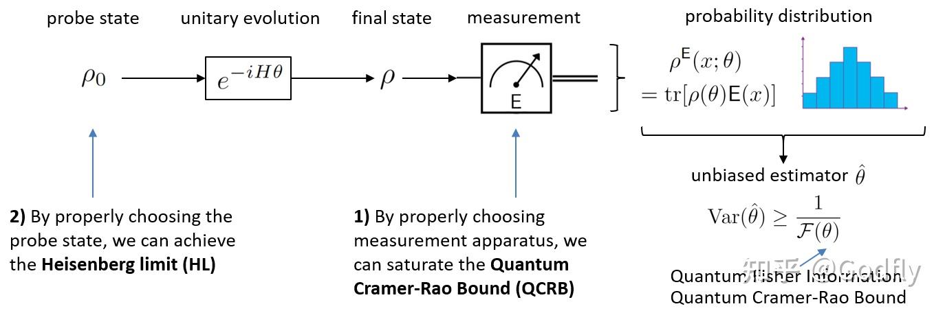
Quantum parameter estimation

Now that we have such powerful tools, from the next section onward, let us apply them to some practical problems.

V. Quantum Phase Estimation

Earlier, we mentioned quantum phase estimation, namely:

Quantum phase estimation: Given a unitary transformation, determine the phases of its eigenvalues.

If the Hilbert space under consideration is n-dimensional, there are (n-1) phases to estimate (the global phase is unimportant).

We have not yet addressed quantum estimation with multiple parameters (we will introduce it in the appendix). Below, we consider the case of only one parameter. There are two such cases: two-level systems and harmonic-oscillator systems.

Why care about quantum phase estimation? Many quantum metrology tasks are accomplished by discriminating the phase of light. If the phase is encoded in a polarization state, it is a two-level system (the two polarization directions of light have an \(SU(2)\) structure). If the phase is encoded in a path (an interferometer), it is a harmonic-oscillator system (the Hamiltonian of the optical field is that of a harmonic oscillator).

5.1 Two-Level Systems

5.1.1 Single-Particle Systems

We now consider a two-level system with Hamiltonian \(\hat{H} = \frac{\hat{Z}}{2}\), and the initial state of the system is a pure state, namely \(|\psi(\theta)\rangle = e^{-i \frac{\hat{Z}}{2}\theta} |\psi_0\rangle \).

The quantum Fisher information is then:

\[ \begin{aligned} F(\theta) &= 4 \left(\Delta \frac{\hat{Z}}{2}\right)^2 = (\Delta \hat{Z})^2 \\ &= \left\langle \psi_0 \left| \hat{Z}^2 \right| \psi_0 \right\rangle - \left\langle \psi_0 \left| Z \right| \psi_0 \right\rangle^2 \\ &= 1 - \left\langle \psi_0 \left| \hat{Z} \right| \psi_0 \right\rangle^2 \end{aligned}\]

To maximize the quantum Fisher information, we require \(\left\langle \psi_0 \left| \hat{Z} \right| \psi_0 \right\rangle = 0\); in other words, \(|\psi_0\rangle\) should lie on the equator of the Bloch sphere. This also accords with our intuition: the closer the initial state is to the equator, the more pronounced the change of the initial state caused by rotation of the Bloch sphere. If the initial state is at the south or north pole, the Fisher information is zero; that is, the initial state senses no rotation at all.

Choosing either the observable \(X\) or \(Y\) can attain the quantum CR lower bound. We may as well directly choose the observable to be \(|0\rangle\langle 1|=X + i Y\) (although this is not an observable, we can measure X and Y separately and combine the results into a complex number). Its expectation value is \(e^{i\theta}\) and its variance is 1. Then \(1 =|\Delta e^{i\theta}| = |ie^{i\theta}\Delta\theta| = \Delta \theta\). That is, \(\Delta \theta = \frac{1}{F(\theta)}\), attaining the CR lower bound.

5.1.2 Multi-Particle Systems

We now consider a two-level system of N particles, with Hamiltonian

\(\hat{H} = \frac{\hat{J_z}}{2} = \sum_k \frac{\hat{Z}_k}{2} = \frac{\hat{Z}}{2} \otimes \hat{\mathbb{I}} \otimes \cdots\otimes \hat{\mathbb{I}} + \hat{\mathbb{I}} \otimes \frac{\hat{Z}}{2} \otimes \cdots\otimes \hat{\mathbb{I}} + \cdots + \hat{\mathbb{I}} \otimes \hat{\mathbb{I}} \otimes \cdots\otimes\frac{\hat{Z}}{2} \).

The quantum Fisher information is then:

\[\begin{aligned} F(\theta) &= \left\langle\left(\sum_k \hat{Z}_k\right)^2\right\rangle - \left\langle\left(\sum_k \hat{Z}_k\right)\right\rangle ^2 \\ &= N+ \left\langle 2\sum_{k \gt l} \hat{Z}_k \hat{Z}_l \right\rangle -\left\langle\left(\sum_k \hat{Z}_k\right)\right\rangle ^2 \\ \end{aligned}\]

To maximize the quantum Fisher information, we need \(\left\langle\left(\sum_k \hat{Z}_k\right)\right\rangle ^2\) to be zero and \(\left\langle \sum_{k \ne l} Z_k Z_l \right\rangle\) to be maximal.

What is the maximum value of \(\left\langle \sum_{k \ne l} Z_k Z_l \right\rangle\)? \(\left\langle Z_k Z_l \right\rangle\) is called the two-body correlator, representing the correlation of Pauli operators between two qubits. Its range is from -1 to 1, and its maximum is 1, meaning that the Z components of the two qubits are always aligned; its minimum is 1, meaning that the Z components of the two qubits are always opposite. Therefore, the maximum value of \(\left\langle \sum_{k \ne l} Z_k Z_l \right\rangle\) is \(N(N-1)/2\). Substituting this into the Fisher information gives:

\[\begin{aligned} F(\theta) &= N+ \left\langle 2\sum_{k \gt l} Z_k Z_l \right\rangle -\left\langle\left(\sum_k \hat{Z}_k\right)\right\rangle ^2 \\ &\le N+N(N-1)-0 \\ &=N^2 \end{aligned}\]

Clearly, at the Heisenberg limit, quantum Fisher information equals the square of the particle number, and the measurement error is inversely proportional to the particle number \(\Delta \theta = \frac{1}{N}\). Therefore, people usually use the Heisenberg limit as a synonym for “error inversely proportional to the particle number.”

What kind of state can reach the Heisenberg limit? The tensor-product state \(|\Psi\rangle = \left(\frac{|0\rangle + |1\rangle}{2}\right)^{\otimes N}\) certainly cannot, because its two-body correlator is zero. In this case, the quantum Fisher information is \(F(\theta) =N\), and the measurement error is inversely proportional to the square root of the particle number \(\Delta \theta = \frac{1}{\sqrt{n}}\). This is called the shot-noise limit.

The maximally entangled state (GHZ state) \(|\Psi\rangle = \frac{|0\rangle^{\otimes N} + |1\rangle^{\otimes N}}{2}\) can reach the Heisenberg limit because all its two-body correlators are one.

Clearly, entanglement and correlation are the core of quantum metrology!

After unitary encoding, the maximally entangled state becomes \(|\Psi\rangle = \frac{|0\rangle^{\otimes N} + e^{i N \theta} |1\rangle^{\otimes N}}{2}\). Choosing the observable \((|0\rangle\langle1|)^{\otimes N}=(X+iY)^{\otimes N}\), its expectation value is \(e^{i N\theta}\) and its variance is 1. \(1 =|\Delta e^{i N \theta}| = |iNe^{i\theta}\Delta\theta| = N\Delta \theta\), namely \(\Delta \theta = \frac{1}{N}\), attaining the Heisenberg limit.

5.2 Harmonic-Oscillator Systems

We now consider a harmonic-oscillator system with Hamiltonian \(H = \hat{N} = \hat{a}^\dag \hat{a}\). The corresponding unitary transformation is \(e^{i\hat{N}\theta} = \sum_{k=0}^{\infty} e^{i N \theta} |N\rangle\langle N|\)

The quantum Fisher information is then:

\[\begin{aligned} F(\theta) &= 4 \left(\Delta \hat{N}\right)^2 \\ &= 4 [\langle \psi | \hat{N}^2 | \psi \rangle - \langle \psi | \hat{N} | \psi \rangle^2] \end{aligned}\]

Clearly, this is in fact the particle-number–phase uncertainty principle:

\[\Delta\theta \Delta N \ge \frac{1}{2}\]

Next, we discuss different initial states (probe states) by category.

5.2.1 Number States

Number state \(| \psi_0 \rangle = | N \rangle\)

The quantum Fisher information is then \(F(\theta) = 0\).

This is easy to understand, because the phase of a number state is completely random (according to the particle-number–phase uncertainty principle, a definite particle number means a completely uncertain phase). Clearly, number states cannot be used to detect phase.

5.2.2 Coherent States

Coherent state \(|\psi_0 \rangle = | \alpha \rangle\)

The quantum Fisher information is then \(F(\theta) = 4 |\alpha|^2 = 4 \bar{n}\).

The CR lower bound on the measurement error is then \(\Delta \theta \ge \frac{1}{2 \sqrt{\bar{n}}}\). This is the shot-noise limit. It follows from the particle-number–phase uncertainty relation.

However, we generally do not call this the Heisenberg limit, but rather the shot-noise limit or the standard quantum limit. The literature often distinguishes this from the Heisenberg limit. This is because we can further increase \(\Delta N\) and thereby reduce \(\Delta \theta\). Only when \(\Delta N\) is proportional to \(\bar{n}\), namely, when \(\Delta \theta \sim \frac{1}{\bar{n}}\), do we call the situation the Heisenberg limit.

Can \(\Delta N\) be proportional to a higher power of \(\bar{n}\)? For example, can \(\Delta N\) be proportional to \(\bar{n}^2\)? Quantum statistics tells us that it cannot. \(\Delta N\) can be at most proportional to \(\bar{n}\).

This is because \((\Delta N)^2 = (g^{(2)}(0)-1)\langle \hat{N}\rangle^2 + \langle \hat{N}\rangle\), where \(g^{(2)}\) is the second-order correlation function, whose value at \(t=0\) is fixed. Clearly, when \(g^{(2)}(0) \gt 1 \), namely, when using bunched light, we have \(\Delta N \propto \langle \hat{N}\rangle = \bar{n}\). However, the \(g^{(2)}(0)\) of a coherent state is exactly 1, so there is only \(\Delta N \propto \sqrt{\bar{n}}\).

Interestingly, thermal radiation has \(g^{(2)}(0)=2\). That is, disordered thermal radiation is more favorable for phase estimation than coherent laser light (counterintuitive, right?) [1]!

From this perspective, the reason people do not call the Heisenberg limit of coherent states the Heisenberg limit is that the Heisenberg limit of bunched light is better than it.

Below is an intuitive illustration for understanding the particle-number–phase uncertainty principle.

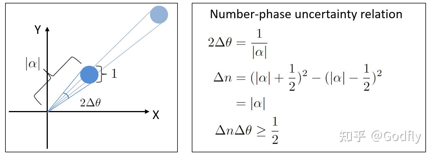
In phase space, a coherent state is a Gaussian function with a standard deviation of 1. Simple geometry gives the particle-number–phase uncertainty principle.

5.2.3 NOON States

In the multi-particle two-level system (Section 5.1.2), we learned that entanglement and correlation must be used to reach the Heisenberg limit. We now construct a particle-number-entangled state.

A NOON state is a particle-number-entangled state \(|\Psi_0\rangle = \frac{|N\rangle \otimes |0\rangle + |0\rangle \otimes |N\rangle}{2}\).

In a NOON state, we in fact introduce an ancilla system and entangle the probe state with the ancilla: when the probe has n photons, the ancilla has zero photons, and vice versa. The overall Hamiltonian is then \(\hat{N} \otimes \mathbb{I}\).

The quantum Fisher information is then:
\(F(\theta) = 4 [ \langle \Psi_0 | (\hat{N} \otimes \mathbb{I})^2 | \Psi_0 \rangle - \langle \Psi_0 | \hat{N} \otimes \mathbb{I} | \Psi_0 \rangle^2 ] = N^2\).

Unlike coherent states, NOON states can reach the Heisenberg limit \(\Delta \theta = \frac{1}{N}\). Choose the observable \(N_X + iN_Y\), where \(N_X = |+ \rangle\langle +| - |-\rangle\langle - |\), \(N_Y = |+i \rangle\langle +i| - |-i\rangle\langle -i |\), and \(|\pm\rangle = \frac{|N\rangle \otimes |0\rangle \pm |0\rangle \otimes |N\rangle}{\sqrt{2}}\), \(|\pm i\rangle = \frac{|N\rangle \otimes |0\rangle \pm i |0\rangle \otimes |N\rangle}{\sqrt{2}}\).

Readers may verify that the expectation value of this observable is \(e^{iN\theta}\) and its variance is 1. Thus \(1=|\Delta e^{iN\theta}| = |iN e^{iN\theta} \Delta \theta| = N\Delta \theta\), namely \(\Delta \theta = \frac{1}{N}\), attaining the Heisenberg limit.

5.2.4 Squeezed States

We will not give explicit formulas for squeezed states here, because they are not very helpful for understanding squeezed states. In fact, you can understand squeezed states without formulas. See the figure below.

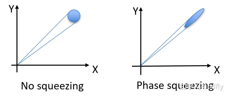
Phase squeezing

In phase space, a coherent state is a Gaussian function with a standard deviation of 1. A squeezed state is actually a coherent state “flattened” along one quadrature, changing from a circle into an ellipse. A squeezed state still satisfies the uncertainty principle; it merely has greater uncertainty in one direction and less uncertainty in the other, with their product fixed (this can also be understood as the area of the ellipse remaining unchanged). Through Phase squeezing as shown above, we can increase \(\Delta N\) and thereby reduce \(\Delta \theta\). Conversely, if we want to reduce \(\Delta N\), we can do so by increasing \(\Delta \theta\); this is Amplitude squeezing.

For amplitude-squeezed states, \(g^{(2)}(0)\lt 1\), whereas for phase-squeezed states, \(g^{(2)}(0) \gt 1\). Recall that we have \((\Delta N)^2 = (g^{(2)}(0)-1)\langle \hat{N}\rangle^2 + \langle \hat{N}\rangle\). Clearly, for squeezed states, \(\Delta N \propto \bar{n}\), \(\Delta \theta \propto \frac{1}{\bar{n}}\), attaining the Heisenberg limit. The greater the squeezing strength, the larger \(g^{(2)}(0)\) becomes, and the higher the proportionality coefficient \(k\) of \(\Delta \theta \sim \frac{1}{k\bar{n}}\) becomes.

Compared with fragile NOON states, squeezed states are more practical. As introduced at the beginning of this article, the famous gravitational-wave detector LIGO uses squeezed states. In addition, when the sample damage threshold is low (for example, biological samples), we cannot reduce shot noise by increasing laser power. In this case, people also use squeezed states to further improve imaging precision without increasing power.

A single-mode squeezed state is not an entangled state, because entanglement can only occur between multiple modes. But why can a single-mode squeezed state reach the Heisenberg limit?

The analysis of multi-particle two-level systems (Section 5.1.2) shows that the essence of increasing quantum Fisher information lies in correlation. Entanglement is merely one way to produce correlation. A single mode can also produce correlation: phase-squeezed states have significant particle-number correlations. Put simply, when the particle number is large, the particle number is large; when the particle number is small, the particle number is small (which sounds like nonsense). This is the property of bunched light, which has a large second-order correlation function. This is analogous to the two-body correlation function in multi-particle two-level systems (Section 5.1.2).

To some extent, the correlation of a single mode can be regarded as the entanglement of that mode with itself.

Summary The analyses of two-level systems and harmonic-oscillator systems show that the way to reduce phase variance is to increase the variance of the generator. In two-level systems, the generator is the angular-momentum operator; in harmonic-oscillator systems, the generator is the particle number N. The way to increase the variance of the generator is to increase its two-body/second-order correlation. In the multimode case, entanglement is one way to increase correlation. Therefore, entanglement and correlation are the core of quantum metrology.

5.3 Interferometers

In 1972, Rainer Weiss proposed a laser-interferometric gravitational-wave detector.

In 1981, Carlton Caves analyzed various quantum noises in interferometers [2], and for the first time proposed using squeezed states to reduce this noise, thereby helping to detect gravitational waves.

In 2002, LIGO was completed and began operation, but no gravitational waves were detected during the following eight years.

In 2010, LIGO was shut down to begin sensitivity-improvement upgrades.

In 2015, Advanced LIGO was completed and began operation. Its sensitivity was four times that of the original LIGO. In the same year, Advanced LIGO detected the first gravitational-wave signal.

In 2017, the Nobel Prize was awarded to Rainer Weiss, Kip Thorne, and Barry Barish in recognition of their “decisive contributions to the LIGO detector and the observation of gravitational waves.”

In 2019, LIGO used squeezed states to further improve its sensitivity by 65%.

Interferometers measure physical quantities related to phase differences by measuring the phase difference. For example, gravitational waves cause changes in the lengths of interferometer arms, thereby producing a phase difference; this is the principle of LIGO.

What kinds of quantum noise exist in interferometers? Clearly, first there is shot noise inversely proportional to the square root of the particle number, which has been analyzed above. In addition, we need to ensure that the detected phase difference is entirely caused by gravitational waves, but this is impossible because photons have momentum. Photons strike mirrors, causing changes in the arm-length difference. This change is proportional to the difference in photon number between the two arms \(\hat{n}_2-\hat{n}_1\). Its expectation value is zero, but its variance is nonzero, namely:

\[ \begin{aligned} \langle (n_2 - n_1)^2 \rangle &= \langle (b_2^\dag b_2 - b_1^\dag b_1)^2 \rangle \\ &= \left\langle \left(\frac{a_2^\dag - a_1^\dag}{\sqrt{2}}\frac{a_2 - a_1}{\sqrt{2}} - \frac{a_2^\dag + a_1^\dag}{\sqrt{2}} \frac{a_2 + a_1}{\sqrt{2}}\right)^2 \right\rangle \\ &= \langle (a_1^\dag a_2 + a_2^\dag a_1)^2 \rangle \\ &= \langle a_1^{\dag 2} a_2^2 \rangle + \langle a_1^2 a_2^{\dag 2}\rangle + \langle a_1^\dag a_1 a_2 a_2^\dag \rangle + \langle a_1 a_1^\dag a_2^\dag a_2 \rangle \\ &= 0 + 0 + |\alpha|^2 + 0 \\ &= |\alpha|^2 \end{aligned}\]

where \(a_1,a_2\) are respectively the two input modes of the beam splitter, corresponding respectively to the laser and vacuum fields; \(b_1,b_2\) are respectively the two output modes of the beam splitter.

Clearly, due to interference between the vacuum field and the laser, the photon-number difference has fluctuations proportional to the square root of the particle number.

In his 1981 paper [2], Carlton Caves pointed out that there are two types of noise in an interferometer: one inversely proportional to the square root of the particle number and one proportional to the square root of the particle number. The former is shot noise, while the latter is radiation-pressure noise. Since these two noises have different origins, the total noise equals their quadrature sum:

\[\Delta L = C_1\frac{1}{\sqrt{\bar{n}}}+C_2 \sqrt{\bar{n}}\]

where \(C_1,C_2\) is a proportionality coefficient with dimensions of length. The minimum noise is thus:

\[\Delta L \ge \sqrt{ C_1\frac{1}{\sqrt{\bar{n}}}\cdot C_2 \sqrt{\bar{n}}} = \sqrt{C_1 C_2}\]

and the minimum noise is attained when \(\bar{n} = \frac{C_1}{C_2}\).

However, substituting typical values of \(C_1, C_2\) reveals that the required \(\bar{n}\) is extremely large, meaning that very high laser power is required, which presents engineering challenges. In other words, the dominant noise is shot noise, so the main means of reducing noise is still to increase laser power.

Caves came up with a way that does not require increasing laser power: rather than increasing laser power to reach the optimal power, one could reduce the optimal power. He proposed using squeezed states to reduce shot noise at the cost of increased radiation-pressure noise. Of course, because radiation-pressure noise is already much smaller than shot noise, the sharp decrease in shot noise produces only a small increase in radiation-pressure noise. One then finds that the optimal laser power is greatly reduced compared with before squeezing.

Thirty-eight years later, people realized his idea.

VI. Standard Quantum Limit (SQL) and Heisenberg Limit (HL)

6.1 The Relationship Between the SQL and Independent Repeated Experiments

From the examples in the previous chapter, you have already understood the Heisenberg limit and the standard quantum limit. Now let us investigate them more carefully.

The standard quantum limit (SQL) can be obtained through simple independent repeated experiments. Let the error in the i-th experiment be \(\Delta x_i\); then the error of the mean \(\bar{x} = \sum_i x_i /N\) is \(\Delta \bar{x}=\Delta x_i/\sqrt{N}\). From this perspective, the standard quantum limit is actually a misnomer—it is not quantum at all.

The derivation is as follows:
\(\begin{aligned} (\Delta \bar{x})^2 &= (\Delta\sum_i x_i / N)^2 \\ &= \Delta(\sum_i x_i)^2 / N^2 \\ &= (\sum_i (\Delta x_i)^2 + \cancel{\sum_{i \ne j} \Delta (x_i x_j)})/N^2 \\ &= \sum_i (\Delta x_i)^2 / N^2 \\ &= (\Delta x_i)^2 / N \end{aligned}\)
The penultimate equality holds because the experiments have no correlation with one another and are mutually independent, namely \(\Delta (x_i x_j) =0\).

The reason this derivation holds is that a separable state of N particles is equivalent to N independent repeated experiments, while the minimum-variance unbiased estimator for independent repeated experiments is the mean of N random variables.

Can this derivation be extended to the Heisenberg limit? Unfortunately, it cannot. For entangled states, the minimum-variance unbiased estimator is no longer the mean, but some other nonlocal function.

Some literature writes the QCRB as \((\Delta \theta)^2 \ge \frac{1}{\sqrt{n}F(\theta)}\), where \(n\) is the number of independent repeated experiments. Take care not to confuse this with the standard quantum limit. The standard quantum limit applies to separable states. A single experiment with a separable state is merely equivalent to independent repeated experiments, but is itself still a single experiment.

6.2 Why the HL Is Proportional to N Squared

Why is the Heisenberg limit proportional to N squared rather than N cubed or even N to the fourth power? This is dictated by the law of energy conservation.

Consider the QFI for a pure state: \(F(\theta) = 4\langle\psi| H^2 |\psi\rangle - 4\langle\psi| H |\psi\rangle^2\). Since energy is proportional to particle number, the first term is proportional to the square of the particle number, while the second term is nonpositive. Therefore, the QFI can be at most proportional to N squared.

For clarity, let us write once again the previous results for two-level systems and harmonic-oscillator systems for readers to appreciate:

Two-level system:

\[\begin{aligned} F(\theta) &= N+ 2\left\langle \underbrace{\sum_{k \gt l} \hat{Z}_k \hat{Z}_l}_{ \frac{N(N-1)}{2} \text{ terms}} \right\rangle -\left\langle\left(\sum_k \hat{Z}_k\right)\right\rangle ^2 \\ \end{aligned}\]

Harmonic-oscillator system:

\[F(\theta)/4 = \langle \hat{N}\rangle + g^{(2)}(0)\langle \hat{N}\rangle^2 - \langle \hat{N}\rangle^2 \]

VII. Quantum Imaging

Quantum imaging is mainly divided into two aspects: improving spatial resolution and improving the signal-to-noise ratio.

7.1 Improving Spatial Resolution

The highest spatial resolution is determined by the diffraction limit. The diffraction limit tells us that the minimum resolvable length equals \(\frac{\lambda}{n \sin \theta}\), where \(\lambda\) is the wavelength, \(\theta\) is the aperture angle (see the figure below), and \(n\) is the refractive index of the medium before the aperture. Next, we derive the diffraction limit using the Heisenberg uncertainty principle.

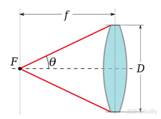
The principle of imaging is that light rays originating from one point converge at another point. When these rays converge at the other point, their momentum information is lost. The amount of lost momentum information determines the position resolution, as given by the Heisenberg uncertainty principle: \(\Delta x\Delta p \ge \frac{\hbar}{2}\).

Now consider the x direction. The lost momentum information is \(\Delta p =p \sin \theta = n \frac{\hbar}{\lambda}\). Therefore, the minimum resolvable length in the x direction is \(\Delta x= \frac{\hbar}{2 \Delta p} = \frac{\lambda}{n \sin \theta}\). This is the diffraction limit.

(To be continued…)

7.2 Improving Signal-to-Noise Ratio

VIII. Other Quantum Parameter Estimation Problems

8.1 Gain & loss sensing

8.2 Noise sensing

8.3 Quantum Parameter Estimation Based on Markovian Dynamics

8.4 Distributed quantum sensing

Appendix: Fisher Information and the CR Lower Bound for Multiple Parameters

This article was created and published using Zhihu On VSCode

References

1. ^Tan, Peng Kian, et al. “Practical Quantum Sensing with Thermal Light.” arXiv preprint arXiv:2303.12338 (2023). https://arxiv.org/pdf/2303.12338.pdf
2. ^abCaves, Carlton M. “Quantum-mechanical noise in an interferometer.” Physical Review D 23.8 (1981): 1693. https://journals.aps.org/prd/abstract/10.1103/PhysRevD.23.1693