Why Does Phase Space Sometimes Look Like a Complex Plane?
 Haifei
Students who have studied physics all know phase space, which consists of generalized coordinates \(q\) and generalized momenta \(p\).
Example 1: The angle of a simple pendulum forms a configuration space \(S_1\). The angle and angular momentum form a phase space \(S_1 \times \mathbb{R}\).
Example 2: Given the Hamiltonian and boundary conditions of a classical electromagnetic field, the electric field amplitude of a certain mode forms a configuration space, while the cosine and sine components of the electric field amplitude in that mode form a phase space.
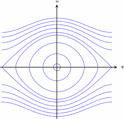
Phase-space trajectory of a simple pendulum
In fact, given a configuration space \(M\), the phase space is the cotangent bundle \(T^*M\) over \(M\).
However, when solving problems, we physicists also often use the complex plane.
Example 1: Given the Hamiltonian equations of a harmonic oscillator
\(\begin{cases} \frac{\mathrm{d}q}{\mathrm{d}t} = \omega p\\ \frac{\mathrm{d}p}{\mathrm{d}t} = -\omega q \end{cases}\)
that is,
\(\frac{\mathrm{d}}{\mathrm{d}t} \begin{bmatrix} q \\ p \end{bmatrix} = \begin{bmatrix} 0 & \omega \\ -\omega & 0 \end{bmatrix} \begin{bmatrix} q\\ p \end{bmatrix}\)
Diagonalization yields the eigenvector \(a^{\pm} = q\pm\mathrm{i}p\), so the derivative of \(a^{\pm}\) depends only on itself:
\(\frac{\mathrm{d}a^{\pm}}{\mathrm{d}t}=\mp\mathrm{i}\omega a^{\pm},\quad a^{\pm}=a_0^{\pm} \exp (\mp\mathrm{i}\omega t)\)
Although there are no complex numbers in classical mechanics, it is very natural for complex numbers to appear here as eigenvalues. Quantizing this method yields the creation and annihilation operators.Example 2: The phasor diagram describing a single-mode classical electromagnetic field is defined on the complex plane. Of course, it can also describe quantities such as current and voltage.
Example 3: The Wigner function describing a single-mode quantum electromagnetic field is defined on the complex plane.
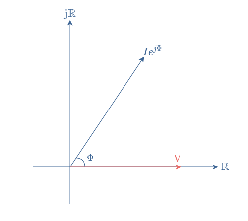
A phasor diagram can be used to solve circuit problems
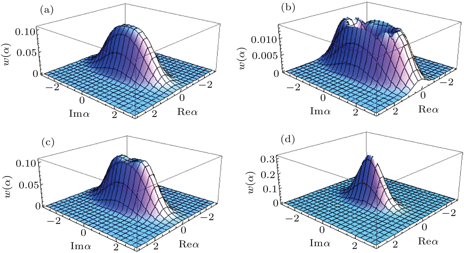
Wigner function
All of these suggest: could phase space be a complex plane? After discussing this with students from the mathematics department, the answer is indeed yes, but only if the phase space itself is a vector space. The argument is as follows:
(1) Phase space is the cotangent bundle of configuration space.
(2) Every cotangent bundle comes equipped with a canonical symplectic structure.
In other words, the tangent space at every point of a cotangent bundle comes equipped with a canonical symplectic form.
(3) If the cotangent bundle itself happens to also be a vector space, then its tangent space is naturally isomorphic to itself. Thus, according to (2), the cotangent bundle is also a symplectic vector space.
(4) A symplectic vector space \((V,\omega)\) with inner product \(g\) comes equipped with a canonical complex structure \(J\) [1].
The complex structure \(J\) on \(V\) is defined as \(J \in \operatorname{End}(V) \quad\text{s.t.} \quad J^2 = -\operatorname{id}\).
From (1-4), we see that if a phase space happens to be a vector space, then that phase space comes equipped with a complex structure.
Therefore, \(T^*\mathbb{R} = \mathbb{R} \times \mathbb{R}^*\) and \(\mathbb{C}\) have the same mathematical structure. \(T^*(\mathbb{R}^n) = \mathbb{R}^n \times (\mathbb{R}^{n})^*\) and \(\mathbb{C}^n\) have the same mathematical structure. This is why we can use the complex plane in place of phase space.
However, note that not all phase spaces can be regarded as complex planes. Only when the configuration space itself is a vector space is the phase space a vector space, and thus can it be regarded as a complex plane. For example, the phase space of a simple pendulum is not a vector space and cannot be regarded as a complex plane.
Update: The discussion in (1-4) above is somewhat abstract. Below is a concrete construction.
Consider the configuration space \(\mathbb{R}\) and phase space \(T^*(\mathbb{R}) = \mathbb{R} \times \mathbb{R}^*\), with global coordinate system \((p,q)\).
The canonical symplectic form on \(T^*(\mathbb{R})\) is \(\omega= \mathrm{d} p \wedge \mathrm{d} q\), which is independent of the basis. Its matrix form is \(M(\omega)=\begin{pmatrix} 0 & 1\\ -1 & 0 \end{pmatrix}\).
The canonical Euclidean inner product on \(T^*(\mathbb{R})\) is \(g = \mathrm{d}q^2 + \mathrm{d}p^2\), and its matrix form is \(M(g)=\begin{pmatrix} 1 & 0\\ 0 & 1 \end{pmatrix}\).
We can use \(g(u,v)=\omega(u,Jv)\) to define the complex structure \(J\in \text{End}[T^*(\mathbb{R})]\). Since its matrix form satisfies \(M(g)=M(\omega)M(J)\), we have \(M(J)=\begin{pmatrix} 0 & -1\\ 1 & 0 \end{pmatrix}\). Does this matrix look somewhat familiar? That’s right: it is the matrix representation of the imaginary unit \(\mathrm{i}\).