Electrodynamics from the Perspective of Gauge Field Theory [Higher and More Elegant Electrodynamics · 2]
 Haifei
If you have not yet read the previous article, please see:
This article uses many concepts from the previous article, so please make sure you have read it.
This article continues to use the metric convention of \((-,+,+,+)\).
Why is electrodynamics a gauge field theory?
To understand what this statement means, we must first understand what electrodynamics is and what gauge field theory is.
I believe most readers have already studied the former, while the latter is what this article aims to emphasize.
Let us begin!
I. What Is a Gauge Transformation (Classical Electrodynamics)
First, what is gauge field theory? A gauge field theory is a theory whose Lagrangian (or, more generally, the physical theory itself) is invariant under local transformations.
Then, what is a local transformation?
For the electromagnetic field, a local transformation is \(\boxed{ A_\mu \mapsto A_\mu + \partial_\mu \lambda }\), which is the covariant form. The contravariant form is the vector we usually refer to: \(A^\mu = g^{\mu\nu}A_\nu\), namely \(A^\mu = (-A_0,A_1,A_2,A_3)\). Therefore, \(A_\mu \mapsto A_\mu + \partial_\mu \lambda \) is equivalent to:
\[\boxed{ \begin{aligned} \phi &\mapsto \phi - \partial_t \lambda \\ \mathbf{A} &\mapsto \mathbf{A} + \nabla \lambda \end{aligned} }\]Students who have studied classical electrodynamics know that this is the electromagnetic gauge transformation, and the actual physics is unaffected before and after the transformation. A gauge transformation is a local transformation because \(\lambda\) is not a constant, but a function of spacetime points.
In classical electrodynamics, we always regard Maxwell’s equations as first principles and gauge transformations as a derivative concept; we regard electric and magnetic fields as fundamental entities, while treating the scalar and vector potentials as convenient mathematical tools with no real physical effects. It is precisely because gauge transformations do not affect electric and magnetic fields that we derived gauge transformations.
But is field strength really the whole story?
No! From a higher perspective, the scalar and vector potentials (the 4-potential) are the fundamental physical entities, while field strength is derivative.
There is physical evidence for this: the Aharonov–Bohm effect (AB effect for short) tells us that the scalar and vector potentials (the 4-potential) have real physical effects. Gauge transformations are not merely a mathematical trick either, but possess a certain ontological status.
The reasons behind all of this must be sought in quantum electrodynamics.
II. What Is a Gauge Transformation (Quantum Electrodynamics)
I believe many readers have heard that the gauge group of the Standard Model is \(U(1) \times SU(2) \times SU(3)\). Among them, \(U(1)\) corresponds to the photon (electromagnetic field), \(SU(2)\) corresponds to weak bosons (W and Z bosons), and \(SU(3)\) corresponds to gluons.
In fact, in quantum electrodynamics, gauge transformations refer to local \(U(1)\) transformations, namely transformations of the form \(\psi(x) \mapsto e^{\mathrm{i}\theta(x)} \psi(x)\), where \(\psi\) denotes the electron wave function, which is a Dirac field.
The difference between a local transformation and a global transformation is that \(\theta\) in a local transformation is itself a field, whereas \(\theta\) in a global transformation is a constant.
Incidentally, according to Noether’s theorem, global \(U(1)\) symmetry implies charge conservation. However, this is not the focus of this article.
If we require the theory to satisfy local symmetry—that is, for the physics to remain invariant under the local transformation \(\psi \mapsto e^{\mathrm{i}\theta}\psi\) —then the electromagnetic field necessarily emerges. In other words, every local gauge symmetry corresponds to a gauge field.
How does this work?
Let us first examine what the local transformation \(\psi \mapsto e^{\mathrm{i}\theta}\psi\) leads to. Since we have not yet specified a Lagrangian, we can only consider quantities related to \(\psi\) itself. For example, \(\partial_\mu \psi\).
We wish that under the local transformation \(\psi \mapsto e^{\mathrm{i}\theta}\psi\), \(\partial_\mu\psi\) transforms in the same way, namely \(\partial_\mu\psi \mapsto e^{\mathrm{i}\theta}\partial_\mu\psi\).
Why do we require \(\partial_\mu\psi\) to transform in the same way as \(\psi\)?
This follows from the Lagrangian of the Dirac field. To keep the Dirac-field Lagrangian \(\mathcal{L}=\bar{\psi}(\mathrm{i}\hbar c \gamma^\mu \partial_\mu -mc^2)\psi \) invariant, we require \(\partial_\mu\psi\) to transform in the same way as \(\psi\).
This can also be seen from the Dirac equation \(\mathrm{i}\hbar \gamma^\mu (\partial_\mu \psi) -mc\,\psi =0\). In fact, the Dirac equation is obtained by varying the action of the Dirac field.
If we substitute \(\psi \mapsto e^{\mathrm{i}\theta}\psi\) into \(\partial_\mu\psi\):
\[\begin{aligned} \partial_\mu \psi \mapsto \partial_\mu(e^{\mathrm{i}\theta} \psi) &= e^{\mathrm{i}\theta}\left[\partial_\mu \psi \color{red}{+ \mathrm{i}(\partial_\mu\theta) \psi}\right] \\ &= e^{\mathrm{i}\theta}\left[(\partial_\mu \color{red}{+ \mathrm{i}\partial_\mu\theta}) \psi\right] \end{aligned}\]we find that the result contains an extra term \( \color{red}{\mathrm{i}(\partial_\mu\theta) \psi}\), so we need to find a way to eliminate it.
Let us introduce \(D_\mu = \partial_\mu - \mathrm{i} (\partial_\mu\theta)\). Then:
\[\begin{aligned} D_\mu \psi \mapsto D_\mu(e^{\mathrm{i}\theta} \psi) &= \left[\partial_\mu \color{red}{- \mathrm{i} (\partial_\mu\theta)}\right] (e^{\mathrm{i}\theta} \psi) \\ &= e^{\mathrm{i}\theta}\partial_\mu \psi \end{aligned}\]Uh… well, this is a little awkward: we have not achieved \(D_\mu\psi \mapsto e^{\mathrm{i}\theta} D_\mu \psi\), but rather \(D_\mu\psi \mapsto e^{\mathrm{i}\theta} \partial_\mu \psi\).
How can we achieve \(D_\mu\psi \mapsto e^{\mathrm{i}\theta} D_\mu \psi\)?
Let us make the term \(\color{red}{-(\partial_\mu\theta)}\) itself into a field \(A_\mu\). What does this mean? It means that we create a new field \(A_\mu\), whose transformation rule is \(A_\mu \mapsto A_\mu \color{red}{- (\partial_\mu\theta)}\).
Next, let \(\boxed{ D_\mu = \partial_\mu + \mathrm{i}A_\mu }\).
Now let us try again:
\[\begin{aligned} D_\mu \psi \mapsto D_\mu^\prime(e^{\mathrm{i}\theta} \psi) &= \left[\partial_\mu + \mathrm{i} (A_\mu \color{red}{- \partial_\mu\theta})\right] (e^{\mathrm{i}\theta} \psi) \\ &= e^{\mathrm{i}\theta}\left(\partial_\mu + \color{red}{\cancel{\mathrm{i}\partial_\mu\theta}} + \mathrm{i}A_\mu - \color{red}{\cancel{\mathrm{i}\partial_\mu\theta}} \right) \psi \\ &= e^{\mathrm{i}\theta}D_\mu \psi \end{aligned}\]We succeeded! The \(D_\mu\) defined in this way is called the covariant derivative.
Note that the covariant derivative here is the covariant derivative on a principal bundle; it is not the same as the covariant derivative \(\nabla_\mu\) on a vector bundle. The latter characterizes the connection between vector-bundle fibers (tangent spaces) and describes the curvature of the manifold itself. The covariant derivative \(D_\mu\) characterizes the connection between principal-bundle fibers and describes the curvature of internal degrees of freedom on the manifold. We will discuss this in detail in Section IV.
Hey, does \(\boxed{A_\mu \mapsto A_\mu \color{red}{- (\partial_\mu\theta)}}\) look somewhat familiar? Is it not precisely the electromagnetic gauge transformation mentioned in Section I?
Or equivalently, \(A \mapsto A - \mathrm{d}\theta\)
In fact, this new field \(A_\mu\) is the electromagnetic field. Its very existence ensures that local gauge transformations do not change the Lagrangian.
To be compatible with SI units, we multiply \(A_\mu\) by a dimensional constant: \(D_\mu = \partial_\mu + \mathrm{i}\frac{e}{\hbar} A_\mu\), thereby ensuring that \(A_\mu\) has the correct dimensions. Here \(e\) is the elementary charge and is positive. Depending on the metric convention and the sign of \(e\), this may also be written as \(D_\mu = \partial_\mu - \mathrm{i}\frac{e}{\hbar} A_\mu\).
In classical electrodynamics, the reason why the Hamiltonian of a charged particle replaces \(\mathbf{p}\) with \((\mathbf{p} - e \mathbf{A})\) is also related to the covariant derivative. Here are several interesting but very simple exercises for the reader:
Replace \(\hat{p}_\mu = -\mathrm{i}\hbar \partial_\mu\) in quantum mechanics with \(\hat{p}_\mu = -\mathrm{i}\hbar D_\mu\) to obtain the canonical momentum \(\mathbf{p} = \mathbf{p}_{\text{kin}} + e\mathbf{A}\), where \(\mathbf{p}_{\text{kin}} = m\dot{\mathbf{x}} = -\mathrm{i}\hbar \nabla\) is the kinetic momentum.
Thus, the energy (Hamiltonian) of a charged particle is:
\(\begin{aligned} H(\mathbf{x},\mathbf{p})&=\frac{1}{2m}(\mathbf{p}_{\text{kin}})^2 + e\phi(\mathbf{x}) \\ &=\frac{1}{2m}[\mathbf{p} - e\mathbf{A}(\mathbf{x})]^2 + e\phi(\mathbf{x}) \end{aligned} \)Use the canonical equations \(\dot{x}^\mu = \frac{\partial H}{\partial p_\mu}, \quad \dot{p}_\mu = -\frac{\partial H}{\partial x^\mu}\) to obtain the Lorentz force: \(\dot{\mathbf{p}}=e(\mathbf{E}+\dot{\mathbf{x}} \times \mathbf{B})\). Note that the particle here carries positive charge \(+e\). For an electron, replace \(+e\) with \(-e\).
Given the Lagrangian \(L(\mathbf{x}, \dot{\mathbf{x}}) = \frac{1}{2} m \dot{\mathbf{x}}^2 + e \dot{\mathbf{x}} \cdot \mathbf{A} - \phi(\mathbf{x})\) of a charged particle, obtain the canonical momentum \(\mathbf{p} = m\dot{\mathbf{x}} + e \mathbf{A}\) through \(p_\mu := \frac{\partial L}{\partial \dot{x}_\mu}\).
Use the Euler–Lagrange equation \(\frac{\partial L}{\partial x^\mu} - \frac{\mathrm{d}}{\mathrm{d}t}\frac{\partial L}{\partial \dot{x}^\mu} = 0\) to obtain the Lorentz force: \(\dot{\mathbf{p}}=e(\mathbf{E}+\dot{\mathbf{x}} \times \mathbf{B})\)
Obtain the Hamiltonian through the Legendre transformation \(H = \mathbf{p} \cdot \dot{\mathbf{x}} - L\) and compare it with the Hamiltonian in 2. They should be identical.
III*. Lagrangians of the Dirac Field and Electromagnetic Field
Readers who are not very familiar with the Dirac equation may skip this section.
Now, substituting \(D_\mu = \partial_\mu + \mathrm{i}\frac{e}{\hbar} A_\mu\) into the Dirac-field Lagrangian \(\mathcal{L}=\bar{\psi}(\mathrm{i}\hbar c \gamma^\mu \partial_\mu -mc^2)\psi \) gives:
\[\begin{aligned} \mathcal{L}_{\text{Dirac}}&=\bar{\psi}(\mathrm{i}\hbar c \gamma^\mu D_\mu-mc^2)\psi \\&=\bar{\psi}(\mathrm{i}\hbar c \gamma^\mu \partial_\mu -mc^2)\psi \color{red}{- eA_\mu c\bar{\psi} \gamma^\mu \psi} \end{aligned}\]Let \(J^\mu = -ec\bar{\psi} \gamma^\mu \psi\) (note that the direction of the current is opposite to the direction of electron motion), giving:
\[\begin{aligned} \mathcal{L}_{\text{Dirac}}&=\bar{\psi}(\mathrm{i}\hbar c \gamma^\mu \partial_\mu-mc^2)\psi \color{red}{+ A_\mu J^\mu} \end{aligned}\]The second term in the expression above is precisely the source term from the previous article:
\[\begin{aligned} \mathcal{L}_{\text{EM}} = -\frac{1}{4\mu_0} F_{\mu\nu} F^{\mu\nu} \color{red}{+ A_{\mu} J^{\mu} } \end{aligned}\]Therefore, the total Lagrangian is:
\[\boxed{ \begin{aligned} &\mathcal{L}[A_\mu, \partial_\nu A_\mu;\psi,\partial_\mu \psi;\bar\psi,\partial_\mu\bar\psi] \\&= \bar{\psi}(\mathrm{i}\hbar c \gamma^\mu \partial_\mu -mc^2)\psi - eA_\mu c\bar{\psi} \gamma^\mu \psi -\frac{1}{4\mu_0} F_{\mu\nu} F^{\mu\nu} \end{aligned} }\]By varying the action \(S=\int\mathcal{L} \mathrm{d}^4x\), one can simultaneously obtain the Dirac equation and Maxwell’s equations. This is the basis of the Lagrangian formulation of quantum electrodynamics.
IV*. Connections on Principal Bundles
In fact, \(A_\mu\) is a connection on a principal bundle. Here, the principal bundle refers to a \(U(1)\)-fiber bundle.
What is a principal bundle? One may imagine a principal bundle as a manifold in which every point comes with a “fiber,” and this fiber has the structure of a Lie group.
Definition of a Lie group: if a manifold is itself also a group, then that manifold is called a Lie group.
The difference between a principal bundle and a vector bundle is that the fibers of a vector bundle are vector spaces, such as tangent/cotangent spaces; whereas the fibers of a principal bundle are Lie groups (strictly speaking, torsors of Lie groups).
For electrodynamics, the principal bundle under consideration has fibers \(U(1)\): you may imagine that a circle grows out of every point on the spacetime manifold. These circles are the fibers we refer to, and they represent phases.
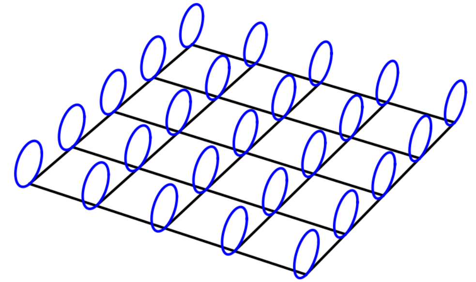
U(1) fiber bundle, image source: generated by ChatGPT
In the figure above, these circles are drawn at discrete points merely for ease of illustration. In reality, every point has such a circle.
A connection on a fiber bundle describes how the fibers are connected to one another. For our \(U(1)\) principal bundle specifically, it is the way the circles in the figure above are connected.
A connection \(A\) on a principal bundle is defined as a Lie-algebra-valued 1-form. Since the Lie algebra of \(U(1)\) is very simple, namely \(\mathbb{R}\), it appears no different from an ordinary 1-form.
Optional reading
Definition of a Lie algebra: a Lie algebra is the tangent space of a Lie group at the identity, together with an additional binary operation on that tangent space, namely the Lie bracket \([\cdot, \cdot]\).
Taking the Lie group \(U(1)\) as an example, the Lie group itself is \(\{\mathrm{e}^{\mathrm{i}\theta} \mid \theta\in[0,2\pi)\}\), while its Lie algebra is \(\mathrm{i}\mathbb{R} = \{\mathrm{i} \theta\mid \theta \in \mathbb{R}\}\). In physics, we usually omit \(\mathrm{i}\) and refer to \(\mathbb{R}\) as the Lie algebra.
From the expression \(A_\mu \mapsto A_\mu - (\partial_\mu\theta)\), we can see that the value of \(\partial_\mu \theta\) as a 1-form should be an element of the Lie algebra.
The Lie bracket on a Lie algebra is induced by the Lie derivative \(\mathcal{L}_V W=[V,W]\) of left-invariant vector fields on the Lie group. Specifically, every element in the tangent space at the identity uniquely corresponds to a left-invariant vector field on the Lie group. Through the Lie bracket between left-invariant vector fields, we can in turn obtain the Lie bracket on the tangent space, thereby making it into a Lie algebra.
The cotangent space naturally has an exterior algebra structure, while the tangent space naturally has a Lie algebra structure.
Curvature is defined as the exterior derivative of the connection: \(F=\mathrm{d}A\). One may imagine that the circles in the figure above are not simply glued together, but glued together in a particular, twisted manner. The curvature of the connection describes precisely this curved way in which the fibers are connected. This can be seen from the transformation rule of \(A\): \(A_\mu \mapsto A_\mu \color{red}{- (\partial_\mu\theta)}\), which describes the change in phase during motion \((\partial_\mu \theta)\).
Let the covariant derivative be \(D_\mu \psi = \partial_\mu \psi +\mathrm{i}A_\mu \psi =0\), and we obtain parallel transport on the principal bundle:
\(\begin{aligned} &D\psi=0\\ &\Rightarrow\left(\partial_\mu + \mathrm{i}\frac{e}{h}A\right) \psi =0 \\ &\Rightarrow \partial_\mu \psi = -\mathrm{i}\frac{e}{\hbar} A_\mu \psi \\ &\Rightarrow \psi(x) = \psi(x_0) \exp\left( -\mathrm{i}\frac{e}{\hbar}\int A_\mu \mathrm{d}x^\mu\right) \end{aligned}\)
We see that, in addition to the dynamical phase \(\int\frac{e}{\hbar}A_0 \mathrm{d}x^0 = \int\frac{1}{\hbar} E \mathrm{d}t\), parallel transport introduces an additional phase \({\int \frac{e}{\hbar} \mathbf{A} \cdot \mathrm{d}\mathbf{l}}\). This is the geometric phase. We will introduce it in later articles in this series.
In other words, the field-strength tensor \(F\) of the electromagnetic field is precisely the curvature of the connection between principal-bundle fibers. This is the geometric meaning of the electromagnetic field as a connection on a principal bundle.
We often say that gravity is a geometric effect. But from the analysis above, electromagnetic force (as well as the weak and strong forces to be introduced below) is also a geometric effect! The former corresponds to a connection on a vector bundle, while the latter correspond to connections on principal bundles.
V*. Yang–Mills Theory
With all this mathematical groundwork, we can now introduce Yang–Mills theory.
The Lagrangian introduced in the previous article:
\[\boxed{ \begin{aligned} \mathcal{L} = -\frac{1}{2} F \wedge (\star F) + A\wedge (\star J) \end{aligned} }\]applies fully in Yang–Mills theory. However, \(A\) here can be not only a connection on a \(U(1)\)-fiber bundle, but also a connection on \(SU(2)\) and \(SU(3)\)-fiber bundles. Their Lie algebras are respectively denoted \(\mathfrak{u}(1), \mathfrak{su}(2), \mathfrak{su}(3)\).
Unlike \(\mathfrak{u}(1)\), which has only 1 generator, \(\mathfrak{su}(2)\) has 3 generators and \(\mathfrak{su}(3)\) has 8 generators; that is, their dimensions are 3 and 8, respectively. In this case, we have \(A_\mu = A_\mu^a T^a\), where \(T^a\) are the generators of the Lie algebra and can serve as a basis for it.
Unlike \(U(1)\), \(SU(2)\) and \(SU(3)\) are noncommutative groups (non-Abelian groups), so gauge field theories based on them are also called non-Abelian gauge field theories.
Due to noncommutativity, curvature is no longer simply \(F=\mathrm{d}A\), but instead \(F=\mathrm{d}A+ A\wedge A\), where \(\wedge\) is the wedge product of differential forms. The reason \(A \wedge A \ne 0\) is also noncommutativity: \(A \wedge A = A_\mu^a A_\nu^b (T^a T^b - T^b T^a) = A_\mu^a A_\nu^b [T^a, T^b]\ne 0 \).
Each generator corresponds to a field, and the corresponding particle is called a gauge boson. For \(U(1)\), the gauge boson is the photon, which mediates the electromagnetic force. For \(SU(2)\), the gauge bosons are \(W^\pm,Z^0\), which mediate the weak force. For \(SU(3)\), the gauge bosons are 8 gluons, which mediate the strong force.
In fact, the electromagnetic and weak forces are not quite this simple. The particle corresponding to \(U(1)\) was originally \(B\), while \(SU(2)\) corresponds to \(W^1,W^2,W^3\). Spontaneous symmetry breaking caused by the Higgs mechanism mixes them together:
\(\begin{aligned} W^\pm &= \frac{W^1 \pm \mathrm{i} W^2}{\sqrt{2}} \\ Z^0 &= W^3 \cos(\theta_W) - B \sin(\theta_W) \\ A &= W^3 \sin(\theta_W) + B\cos(\theta_W) \end{aligned}\)
This is how the photon \(A\) and weak bosons \(W^\pm,Z^0\) arise. The specific mechanism will not be introduced here due to space limitations.
The next article in this series