The Electromagnetic Field Is More Than Just Electric and Magnetic Fields—The AB Effect and Berry Connection [Higher and More Elegant Electrodynamics · 3]
 Haifei
Previous article in this series:
The electromagnetic field is not simply the electric field and the magnetic field.
In other words, the electromagnetic field is more than just the electric field and the magnetic field.
What does this mean?
1. Electromagnetic Potentials Have a Higher Status Than Field Strengths
In a previous article, we left a question open:
\(\boxed{\begin{aligned} \phi &\mapsto \phi - \partial_t \lambda \\ \mathbf{A} &\mapsto \mathbf{A} + \nabla \lambda \end{aligned}}\)
Students who have studied classical electrodynamics all know that this is an electromagnetic gauge transformation, and that the actual physics is unaffected before and after the transformation.
In classical electrodynamics, we always regard Maxwell’s equations as first principles and gauge transformations as a derivative concept; we regard electric and magnetic fields as fundamental entities, while treating scalar and vector potentials as convenient mathematical tools with no actual physical effect. It is precisely because gauge transformations do not affect electric and magnetic fields that we derive gauge transformations.
But is field strength really the whole story?
No! From a higher perspective, the electromagnetic potential \(A = (\phi, \mathbf{A})\) is the fundamental physical entity, while field strength is derivative.
You may have many questions: in electrodynamics, aren’t the field strengths \(\mathbf{E}\) and \(\mathbf{B}\) the entirety of the electromagnetic field? Don’t Maxwell’s equations describe changes in field strengths? Aren’t observables limited to field strengths? Given the existence of gauge freedom, isn’t the electromagnetic potential \(A = (\phi, \mathbf{A})\) unobservable?
Indeed, in classical electrodynamics, the above view is entirely correct.
However, upon entering the quantum domain, people gradually discovered that the field strengths \(\mathbf{E}\) and \(\mathbf{B}\) are not the whole story: some phenomena cannot be explained using only \(\mathbf{E}\) and \(\mathbf{B}\), and can be explained only through the electromagnetic potential \(A\).
This phenomenon is the Aharonov–Bohm effect (AB effect for short). Only with the discovery of the AB effect did people formally establish the ontological status of \(A\), regarding the field strengths \(\mathbf{E}\) and \(\mathbf{B}\) as derivative instead.
In quantum electrodynamics, you hardly see \(\mathbf{E}\) and \(\mathbf{B}\) at all. They are replaced by the electromagnetic potential \(A\).
2. The Aharonov-Bohm Effect
Let us now briefly derive the AB effect.
In a previous article, we stated that the covariant derivative is \(D_\mu=\partial_\mu + \mathrm{i}\frac{e}{h}A_\mu\).
Now, let an electron move slowly along a path. Then its covariant derivative should be zero:
\[D_\mu \psi = 0\]This is just as in general relativity, where we set the covariant derivative to zero when parallel transporting a vector.
Thus,
\[\begin{aligned} &D_\mu\psi=0\\ &\Rightarrow\left(\partial_\mu + \mathrm{i}\frac{e}{h}A_\mu\right) \psi =0 \\ &\Rightarrow \partial_\mu \psi = -\mathrm{i}\frac{e}{\hbar} A_\mu \psi \\ &\Rightarrow \psi(x) = \psi(x_0) \exp\left( -\mathrm{i}\frac{e}{\hbar}\int A_\mu \mathrm{d}x^\mu\right) \end{aligned}\]Clearly, in addition to the dynamical phase \(\int\frac{e}{\hbar}A_0 \mathrm{d}x^0 = \int\frac{1}{\hbar} E \mathrm{d}t\), the electron acquires an additional phase \(\color{red}{\int \frac{e}{\hbar} \mathbf{A} \cdot \mathrm{d}\mathbf{l}}\). This is the Aharonov-Bohm phase.
Consider a very long solenoid, with a magnetic field inside but zero magnetic field outside. Now let an electron slowly travel once around it. Compared with when the solenoid is not energized, the phase accumulated by the electron changes by
\[\boxed{\begin{aligned} \Delta \theta = \frac{e}{\hbar}\oint \mathbf{A} \cdot \mathrm{d}\mathbf{l} = \frac{e}{\hbar}\int \mathbf{B} \cdot \mathrm{d}\mathbf{S} = \frac{e }{\hbar}\Phi \end{aligned}}\]where \(\Phi\) is the magnetic flux in the solenoid.
People were astonished to discover that the electron had not passed through any \(\mathbf{E},\mathbf{B}\); in other words, along the electron’s path, \(\mathbf{E}=\mathbf{B}=\mathbf{0}\), yet the electron was still affected by the electromagnetic field! This is because along the electron’s path, although there is \(\mathbf{E}=\mathbf{B}=\mathbf{0}\), the electromagnetic vector potential \(\mathbf{A}\ne 0\).
This tells us that \(\mathbf{A}\) is the fundamental entity, while \(\mathbf{E}\) and \(\mathbf{B}\) are merely derivatives.
Indeed, in a previous article, we mentioned that \(A\), as a connection on a principal bundle, is primary. \(\mathbf{E}\) and \(\mathbf{B}\) (or the electromagnetic tensor \(F = \mathrm{d}A\)), as the curvature of the connection \(A\), are secondary.
Note that \(\Delta \theta = \frac{e}{\hbar}\oint \mathbf{A} \cdot \mathrm{d}\mathbf{l}\) is gauge-invariant: setting \(\mathbf{A} \rightarrow \mathbf{A} + \nabla\lambda\), we have \(\oint \nabla \lambda\cdot \mathrm{d}\mathbf{l} = 0\). Clearly, only the AB phase along a closed path is gauge-invariant.
3. Holonomy
Traveling around a loop on the base manifold of a fiber bundle and returning to the starting point, thereby changing the value in the fiber, is called holonomy. For our \(U(1)\) principal bundle, its fiber is \(U(1)\), and in this case it is an element of \(U(1)\) ( \(\mathrm{e}^{\mathrm{i}\theta}\) ) that changes.
This is like a tangent vector that changes after going around a loop on a sphere and returning to its starting point, because a tangent vector is an element of the fiber (tangent space) of the tangent bundle.
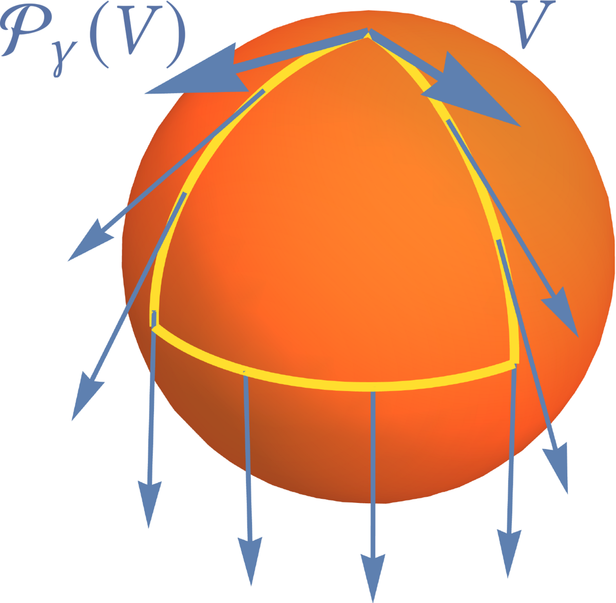
Holonomy on the tangent bundle
In physics, holonomy on a \(U(1)\) fiber bundle has a special name: the geometric phase, or Berry phase. Its corresponding connection is called the Berry connection, and its corresponding curvature is called the Berry curvature.
In the AB effect, the Berry connection \(\mathcal{A}\) is none other than the electromagnetic 1-form \(A\) (in fact, it must also be multiplied by the constant \(e/\hbar\): \(\mathcal{A} = \frac{e}{\hbar} A\)), while the Berry curvature \(F\) is the magnetic field \(B\) (in fact, it must also be multiplied by the constant \(e/\hbar\): \(F = \frac{e}{\hbar} B\)).
More precisely, the Berry curvature should be the exterior derivative \(F = \mathrm{d}A\) of \(A\), and is a 2-form.
Through Hodge duality in three-dimensional Euclidean space, we can dualize a 2-form into a 1-form, namely the magnetic-field 1-form. Taking the exterior derivative of the 1-form \(A\) and then taking its Hodge dual is equivalent to taking its curl: \(\nabla \times A^\sharp = \star\mathrm{d}A\).
The reason the magnetic field is called a pseudovector is also that the magnetic field is essentially a 2-form rather than a 1-form. What we commonly call the magnetic field is actually the Hodge dual of this 2-form.
The electromagnetic potential \(\mathbf{A}\) is merely a connection on a particular \(U(1)\) fiber bundle, whose base manifold is configuration space itself.
There are many other \(U(1)\) fiber bundles whose base manifolds are not configuration space, but abstract parameter spaces such as momentum space. Analysis of the quantum Hall effect is carried out on a \(U(1)\) fiber bundle in momentum space, where we can likewise derive Berry connections and Berry curvatures. These concepts have become central to modern condensed matter physics.
4. Berry Connection/Curvature
Next, let us derive the formula for the Berry connection.
Consider now an abstract base manifold \(M\). A point \(s \in M\) on \(M\) is a parameter of the Hamiltonian \(H(s)\), rather than a spacetime point. Let an eigenstate of the Hamiltonian be denoted by \(\psi\).
Starting from parallel transport:
\[\begin{aligned} &D_\mu\psi=0\\ &\Rightarrow\left(\partial_\mu + \mathrm{i}A_\mu\right) \psi =0 \\ &\Rightarrow \partial_\mu \psi = -\mathrm{i}A_\mu \psi \end{aligned}\]Taking the inner product of both sides above with \(\psi\) gives:
\[\langle\psi | \partial_\mu \psi \rangle = -\mathrm{i} A_\mu \langle\psi | \psi\rangle\]That is:
\[\boxed{A_\mu = \mathrm{i} \langle \psi | \partial_\mu \psi\rangle}\]This is the expression for the Berry connection. It can also be written as:
\[\boxed{\mathbf{A} = \mathrm{i} \langle \psi|\nabla \psi\rangle}\]The Berry curvature is the exterior derivative of the Berry connection:
\[F = \mathrm{d}A\]In index notation, this is
\[ \begin{aligned} F_{\mu\nu} &= \partial_\mu A_\nu - \partial_\nu A_\mu \\ &= \mathrm{i} \left[\partial_\mu \langle \psi | \partial_\nu \psi\rangle -\partial_\nu \langle \psi | \partial_\mu \psi\rangle \right] \\ &= \mathrm{i} [\langle \partial_\mu \psi| \partial_\nu \psi \rangle - \langle \partial_\nu \psi| \partial_\mu \psi \rangle] \end{aligned} \]namely
\[\boxed{F_{\mu\nu}=\mathrm{i} [\langle \partial_\mu \psi| \partial_\nu \psi \rangle - \langle \partial_\nu \psi| \partial_\mu \psi \rangle]}\]The geometric phase is the integral of the connection 1-form \(A\) over a closed curve \(\gamma\):
\[\boxed{ \Delta \theta = \int_\gamma A }\]If there exists a surface \(\Sigma\) such that the curve \(\gamma\) is the boundary of \(\Sigma\), then by Stokes’ theorem,
\[\begin{aligned} \Delta \theta = \int_{\partial \Sigma} A = \int_{\Sigma} \mathrm{d}A = \int_\Sigma F \end{aligned}\]where \(\partial \Sigma\) denotes the boundary of \(\Sigma\).
Thus, the geometric phase can also be obtained by integrating the curvature 2-form \(F\) over the surface \(\Sigma\):
\[\boxed{ \Delta \theta = \int_\Sigma F}\]If we take \(\Sigma\) to be a closed surface, then \(\partial \Sigma=0\), and thus
\[\Delta \theta = \int_\Sigma F = \int_{\partial \Sigma} A = 0\]However, on a topologically nontrivial manifold, this integral is not necessarily zero. This is because a global connection \(A\) cannot be defined in this case, so Stokes’ theorem no longer applies. We will discuss this in detail in the next article.
Note that the geometric phase \(\Delta \theta\) is not an element of \(U(1)\), but an element of the Lie algebra of \(U(1)\) (namely \(\mathbb{R}\)). In other words, the geometric phase takes values not in \(U(1) = \{ e^{\mathrm{i}\theta} \mid \theta \in [0,2\pi) \}\), but in \(\mathbb{R}\). It represents the change in phase, rather than the phase itself. That is, the geometric phase can take values such as \(2\pi, 4\pi\), and these are not equivalent to \(0\).
In a two-dimensional lattice, due to periodic boundary conditions, the electron momentum space \(M\) is a torus, i.e., \(M=T^2\). Integrating the Berry curvature \(F\) over \(T^2\) then yields the Chern number, which need not be zero:
\[\int_{M} F = 2 k\pi\,\,(k\in\mathbb{Z})\]Here \(k\) is the Chern number, defined as \(k = \frac{1}{2\pi}\int_{M} F\).
In the next article, we will introduce the concept of the Chern number and calculate connections, curvatures, and Chern numbers in specific examples.
5*. Non-Abelian Geometric Phase
Previously, we defined the Berry connection through parallel transport:
Starting from parallel transport:
\(\begin{aligned} &D_\mu\psi=0\\ &\Rightarrow\left(\partial_\mu + \mathrm{i}A_\mu\right) \psi =0 \\ &\Rightarrow \partial_\mu \psi = -\mathrm{i}A_\mu \psi \end{aligned}\)
Taking the inner product of both sides above with \(\psi\) gives:
\(\langle\psi | \partial_\mu \psi \rangle = -\mathrm{i} A_\mu \langle\psi | \psi\rangle\)
That is: \(\boxed{A_\mu = \mathrm{i} \langle \psi | \partial_\mu \psi\rangle}\)
This is the expression for the Berry connection. It can also be written as:
\(\boxed{\mathbf{A} = \mathrm{i} \langle \psi|\nabla \psi\rangle}\)
At that time, we considered a \(U(1)\) fiber bundle. However, the above steps also hold completely for a \(U(N)\) fiber bundle! The difference is that the connection \(A\) is now an element of the Lie algebra of \(U(N)\), namely \(\mathfrak{u}(N)\).
Under what circumstances do we consider a \(U(N)\) fiber bundle? When energy levels are degenerate.
The eigenstate considered previously was nondegenerate. In this case, if the parameters of the Hamiltonian are changed slowly, the system will remain in the corresponding eigenstate, with only its phase able to change. The group describing phase changes is \(U(1)\).
But if the eigenstate we consider lies in a degenerate energy level (eigenspace), and the Hamiltonian parameters are changed slowly (in a way that does not break the degeneracy), then although the state of the system remains in the original eigenspace, it can move within that eigenspace. The group describing transformations within the eigenspace is \(U(N)\).
Unlike \(U(1)\), \(U(N)\) is a non-Abelian group, so the corresponding geometric phase, connection, and so on can all be prefixed with “non-Abelian.”
In this case, in \( \partial_\mu \psi = -\mathrm{i}A_\mu \psi\), \(A_\mu\) is no longer an ordinary real number, but a matrix, namely an element of \(\mathfrak{u}(N)\), describing an infinitesimal \(U(N)\) rotation. And \(\psi\) is no longer an eigenvector, but an eigenspace.
We choose a basis for the eigenspace: \(\{ \psi_1, \psi_2, ..., \psi_N\}\). We may then write \( \partial_\mu \psi = -\mathrm{i}A_\mu \psi\) as:
\[ \partial_\mu \psi_b = -\mathrm{i}A_{\mu b}^{c} \psi_c\]Taking the inner product of both sides with \(\psi_a\) gives:
\[\langle \psi_a | \partial_\mu \psi_b \rangle = -\mathrm{i}\langle \psi_a |A_{\mu b}^{c} \psi_c \rangle = -\mathrm{i} A_{\mu b}^a\]Thus,
\[\boxed{ A_{\mu}^{ab} = \mathrm{i}\langle \psi_a | \partial_\mu \psi_b \rangle }\]This is the non-Abelian Berry connection.
The unitary transformation \(U\in U(N)\) induced by parallel transport along the path \(\gamma\) is called the non-Abelian geometric phase:
\[U = \mathcal{P}\exp(\mathrm{i}\int_\gamma A)\]It is the integral of the non-Abelian connection \(A\) along the path \(\gamma\). Here \(\mathcal{P}\) is the path-ordering operator.
Its effect is to order the operator products \(A(t_1)A(t_2)\cdots A(t_N)\) in each term of the Taylor-expanded series according to their order along the path, such that \(t_1 \gt t_2 \gt \cdots \gt t_N\). Ordering is needed because the connections \(A(t_1)\) and \(A(t_2)\) at different points do not commute.
The curvature is calculated as follows (see the appendix):
\[\boxed{ F=\mathrm{d}A+\mathrm{i}A\wedge A }\]namely
\[\boxed{ F_{\mu\nu} = \partial_\mu A_{\nu}-\partial_{\nu}A_{\mu} +\mathrm{i} [A_\mu,A_\nu] }\]Each term in the above expression is a matrix. Written out in expanded form:
\[\boxed{ F_{\mu\nu}^{ab} = \partial_\mu A_{\nu}^{a b} - \partial_\nu A_{\mu }^{ab} +\mathrm{i}( A^{ac}_{\mu } A^{cb}_{\nu} - A_{\nu}^{ac} A_{\mu}^{cb}) }\]Next article in this series:
Why does non-Abelian curvature contain an additional term \(\mathrm{i}A\wedge A\)?
\[F=\mathrm{d}A+\mathrm{i}A\wedge A\]Let us look again at the covariant derivative \(\mathrm{D}\). Abstractly, it is actually a map \(\Omega^n(T^*M) \rightarrow \Omega^{n+1}(T^*M)\) that transforms an n-form into an (n+1)-form, defined as
\[\boxed{ \mathrm{D} = \mathrm{d} +\mathrm{i} A\wedge }\]Now consider the square of the covariant derivative \(\mathrm{D}\). It equals
\[\mathrm{D}^2 = (\mathrm{d} +\mathrm{i} A\wedge)^2 = \mathrm{i}(\mathrm{d} A -\mathrm{i} A\wedge A) \wedge\]Proof:
\[\begin{aligned} \mathrm{D}^2 \psi &= (\mathrm{d} +\mathrm{i} A\wedge)(\mathrm{d}\psi +\mathrm{i} A\wedge\psi) \\ &=\cancel{\mathrm{d}^2\psi} +\mathrm{i} A\wedge \mathrm{d}\psi + \mathrm{d}(\mathrm{i} A\wedge \psi)-A\wedge A\wedge \psi \\ &=\cancel{\mathrm{i} A\wedge \mathrm{d}\psi} + (\mathrm{i} \mathrm{d}A \wedge \psi - \cancel{\mathrm{i} A\wedge \mathrm{d}\psi)}-A\wedge A\wedge \psi \\ &= (\mathrm{i} \mathrm{d}A - A\wedge A)\wedge \psi \\ &= \mathrm{i} (\mathrm{d}A + \mathrm{i}A\wedge A) \wedge \psi \end{aligned}\]We may therefore define the curvature operator as \(F=-\mathrm{i}\ \mathrm{D}^2 =(\mathrm{d}A + \mathrm{i}A\wedge A) \wedge\). It transforms an n-form into an (n+2)-form.